Week 8: The Poisson distribution
Wed, Mar 28, 2018 Made by Judit Kisistók, incorporating some snippets from the solution sheets of Sara Moeskjær and Moisés Coll Maciá. The exercise session was created by Thomas Bataillon and Palle Villesen at Aarhus University.library(ggplot2)Table of contents
Learning goals
By the end of this session, you should be able to…
- master Goodness-of-fit tests:
- What null is tested, what degrees of freedom are appropriate?
- The Poisson probability distribution and its use as a null distribution for randomness of events in space / time
- GOF test using the Poisson as a null model
README FIRST :-)
We first introduce / illustrate THREE important new R functions: dpois(), ppois() and rpois().
You then have to apply these functions in a variety of situations.
It’s a good idea to work sequentially:
1. Try the R new functions especially the one that allows you to visualize and calculate probabilities using the Poisson probablity distributions
2. Try the next questions where you will redo in R the extinction example of Chapter 8 step by step
3. Try the set of Chapter 8 practice and assignment problems listed below (also listed in the weekly note)
4. Try the example where you have to “plan” a sequencing experiment
R functions for simulating from /calculating the Poisson probability distribution
# If you want to draw 100 random numbers from a Poisson distribution with mean 0.1, 1 ..etc
my100deviates=rpois(n = 10^4, lambda = 0.1) ## try to evaluate that several times (you get different numbers)
hist(my100deviates, main="Draws from a Poisson with mean 0.1", col="deeppink4")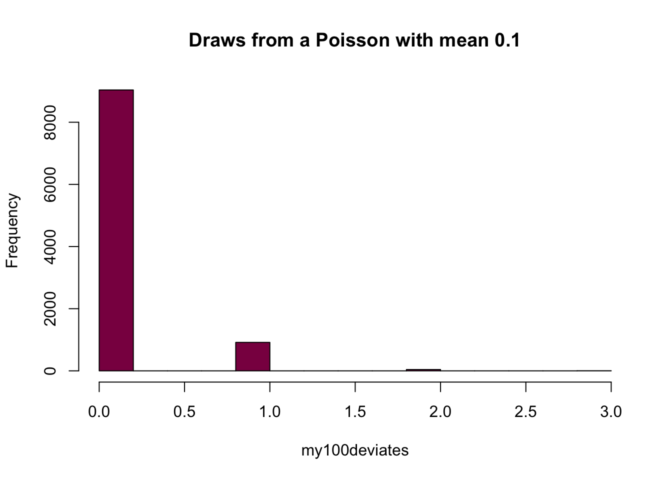
my100deviates=rpois(n = 10^4, lambda = 1) ## try to evaluate that several times (you get different numbers)
hist(my100deviates, main="10^4 draws from a Poisson with mean 1", col="deeppink4")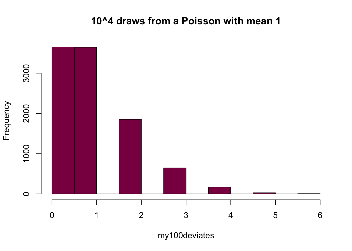
my100deviates=rpois(n = 10^4, lambda = 5) ## try to evaluate that several times (you get different numbers)
hist(my100deviates, main="10^4 draws from a Poisson with mean 5", col="deeppink4")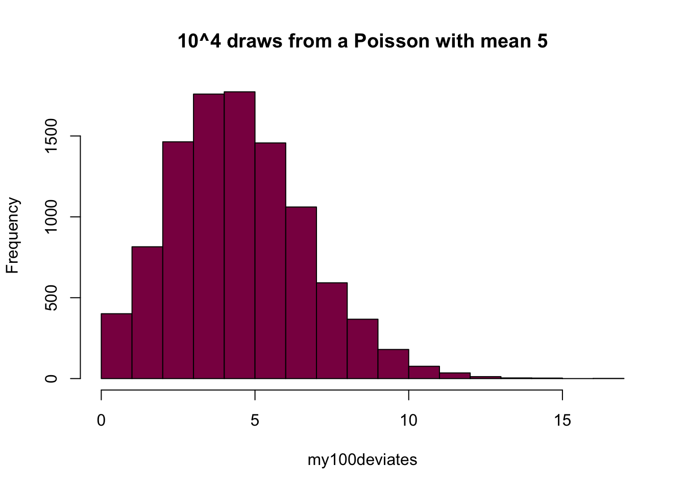
If you want to graph the Poisson probability distribution:
# you have to "plot" the density function over a grid of coordinates (here 0,1,2, etc)
xs= seq(from = 0, to=10, by=1 ) # xs is a vector of coordinates on the X axis
y1=dpois(x = xs, lambda = 0.1) # y1 stores the probabilities of the poisson distribution (mean 0.1) at each X discrete value
y2=dpois(x = xs, lambda = 1) # y2 stores the probabilities of the poisson distribution (mean 1) at each X discrete value
y3=dpois(x = xs, lambda = 5) # y3 stores the probabilities of the poisson distribution (mean 5) at each X discrete value
Did we span the range of probability that matters?
sum(y1) #sums up to 1 - so we have all the probabilities in the range## [1] 1sum(y2) #also sums up to 1## [1] 1sum(y3) #this doesn't have all the probabilities in the range as it sums up to less than 1## [1] 0.9863047Pretty much. While in principle the counts could span to infinity, in practice they fall relatively fast after the mean of the Poisson distribution has been reached. y1 and y2 illustrate this very well - and you could try to plot y3 on a slightly broader range (eg. 25 instead of 10) to see that you’re able to capture the entire probability range.
Visualizing Poisson distributions in R
# Plotting the densities of 3 different Poisson distributions
plot(xs, y1, type ="h", lwd=3, xlab="X ", ylab= "P(X)")  # Plotting the probability of Poisson distribution (mean 0.1)
lines(xs+0.2, y2, type ="h", lwd=3, col="blue")  # adding the probability of Poisson distribution (mean 1) to the previous plot
lines(xs+0.4, y3, type="h", lwd=3, col="magenta")# adding the probability of Poisson distribution (mean 5) to the previous plot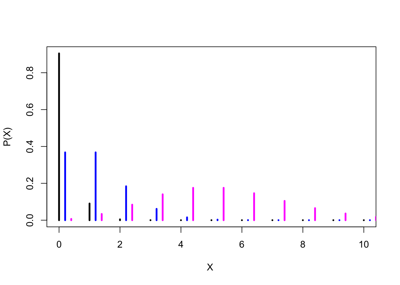
Take me back to the beginning!
Mastering Poisson distribution calculations: example of genome sequencing
Let’s call X a random variable that tracks how many times a nucleotide was sequenced in a genome for a 2X experiment. If sequencing is truly random discuss why it is a fair assumption to assume X is Poisson?
If the sequencing is truly random, that means that whether or not we happen to sequence a nucleotide is independent of any other nucleotide, and that the probability of sequencing a nucleotide is the same over the span of the entire genome. Since we assume that these assumptions are met, we can say that the number of times a nucleotide is sequenced is described by the Poisson distribution.
In “Poisson-talk”, the number of successes is the number of sequenced nucleotides and the blocks of space are the regions in the genome.
What is the probability that a given nucleotide was not sequenced?
In this case, the number of successes is 0 and lambda is 2 because we know that it’s a 2X experiment (so we’d expect every nucleotide to be sequenced 2 times on average).
dpois(x = 0, lambda = 2)## [1] 0.1353353What is the probability that a stretch of 100 bp was missed entirely?
This is equivalent to saying that we are looking for the probability of having 0 successes 100 times in a row - so we can apply the multiplication rule.
(dpois(x = 0, lambda = 2))^100## [1] 1.383897e-87Simulate the distribution of coverage you expect if you had a bactertial genome with:
- 90% of genes with “intermediate” GC content where sequencing was 5X
- 10% of genes with “very low” GC content (because they were recently acquired from a GC poor bacteria) but where sequencing did not work well so only 1X was actually achieved
- Simulate a genome of 5000 genes
To simulate this mixed distribution, we can create the two distributions individually and then concatenate them.
# first of all, we simulate the two distributions that we intend to mix
pois_90 = rpois(n = 5000*0.9, lambda = 5)
pois_10 = rpois(n = 500, lambda = 1)
mixed_pois = c(pois_90, pois_10) # this is our mixed distribution, created by concatenating the pois_90 and pois_10 distributions

# then we put the simulated data into a dataframe - here I create a column called "type" and another called "read counts" and I populate them with the simulated data
gc_data = data.frame(type = c(rep("normal_GC", 5000*0.9), rep("low_GC", 5000*0.1)),
                  read_counts = c(pois_90, pois_10))

# let's plot it in base R
p2 <- hist(pois_90, col = "deeppink4") 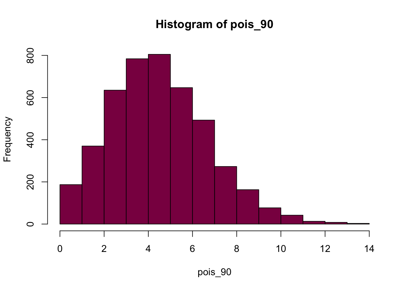
p3 <- hist(pois_10, col = "deeppink4") 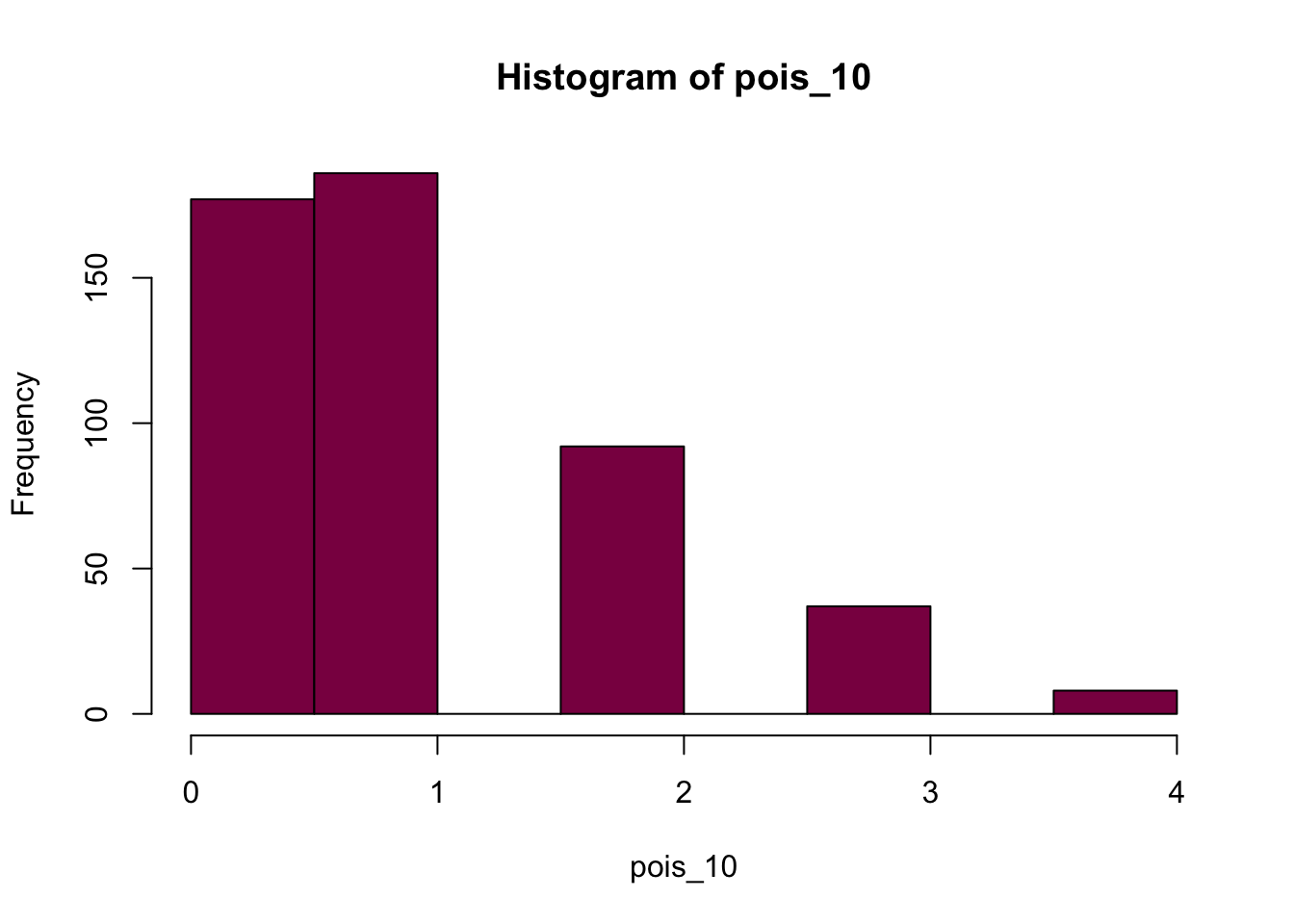
p1 <- hist(mixed_pois, col = "deeppink4")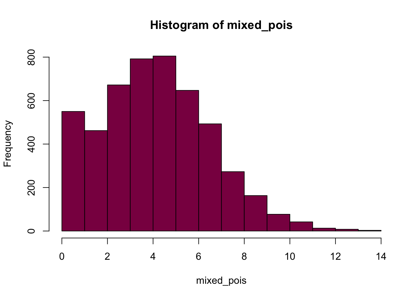
plot(p1, col="darkgreen", xlim=c(0,15))
plot(p2, col="deeppink4", xlim=c(0,15), ylim = c(0,800), xlab="Number of successes", add=T)
# add = T makes sure that you add these plots on top of eachother, and don't just create individual plots
plot(p3, col="cornflowerblue", xlim=c(0,15), add=T) 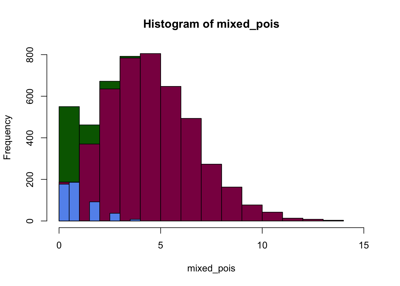
# plot the data from our dataframe
plot(table(gc_data$read_counts), main = "Histogram of reads", xlab = "Number of reads", ylab = "Counts")

# let's superimpose the "clean" Poisson distribution with mean = 5:
points(x = 0:15, y = (dpois(x = 0:15, lambda = 5)*5000*.9), col = "red", type = "b")

# and then the Poisson distribution with mean = 1:
points(x = 0:15, y = (dpois(x = 0:15, lambda = 1)*5000*.1), col = "blue", type = "b")

# neither of these fit perfectly - so let's superimpose the mixed distribution:
points(x = 0:15, y = (dpois(x = 0:15, lambda = 1)*5000*.1)+(dpois(x = 0:15, lambda = 5)*5000*.9),
       col = "green", type = "b")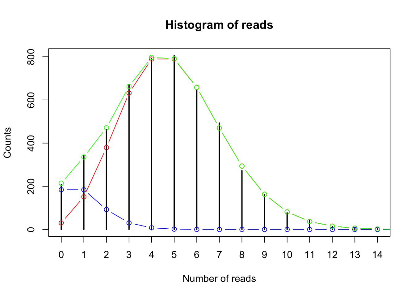
# and this is how we would do it in ggplot
# we plot the data to see how it looks in general - note that this is all the data, so what you see is the mixed distribution
ggplot(gc_data) +
  geom_histogram(aes(x = read_counts, fill = type), binwidth = 1, col = "black") +
  xlab("Number of reads") +
  ylab("Counts")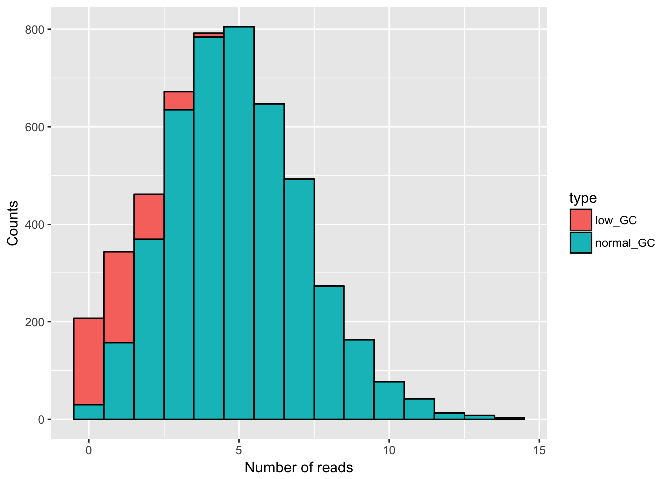
# we can plot the two types individually as well
# first, we filter the data
low_GC_reads = gc_data[gc_data$type == "low_GC",]
normal_GC_reads = gc_data[gc_data$type == "normal_GC",]

# and then we plot - we can see that the individual distributions fit the corresponding histograms well
ggplot() +
  geom_histogram(data = low_GC_reads, aes(x = read_counts, fill = type), binwidth = 1, alpha = .7, col = "black") +
  geom_histogram(data = normal_GC_reads, aes(x = read_counts, fill = type), binwidth = 1, alpha = .7, col = "black") +
  geom_line(data = data.frame(x = 0:13, y = dpois(x = 0:13, lambda = 5)*5000*.9), aes(x = x, y = y)) +
  geom_line(data = data.frame(x = 0:13, y = dpois(x = 0:13, lambda = 1)*5000*.1), aes(x = x, y = y)) +
  geom_point(data = data.frame(x = 0:13, y = dpois(x = 0:13, lambda = 5)*5000*.9), aes(x = x, y = y)) +
  geom_point(data = data.frame(x = 0:13, y = dpois(x = 0:13, lambda = 1)*5000*.1), aes(x = x, y = y))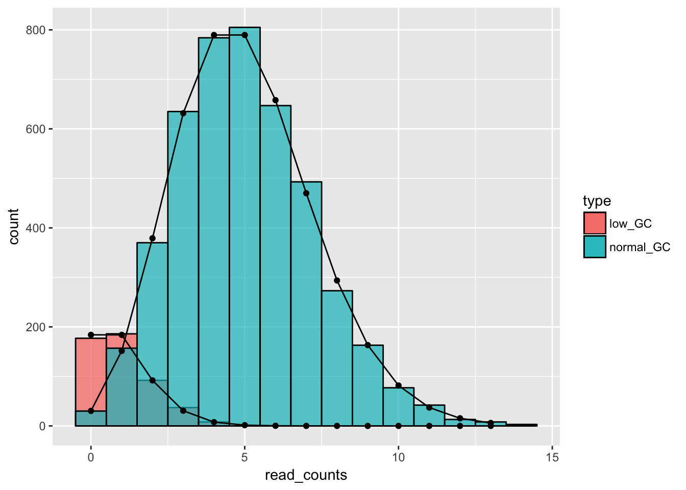
Will this look like a Poisson distribution?
We can see that the distribution that we get is a mixture of different Poisson distributions - which is due to the heterogeneity in the sample. Luckily, in this case we knew what made the data heterogeneous - however, in real experiments it might not be this clear-cut so it can be a challenge finding out what biological factor modifies our expected distribution.
Take me back to the beginning!
Example 8.6 of the book “Extinctions” in R
# Here is where you can get the original data
library(abd)
extinctData <- read.csv(url("http://whitlockschluter.zoology.ubc.ca/wp-content/data/chapter08/chap08e6MassExtinctions.csv"))
head(extinctData)
## numberOfExtinctions
## 1 1
## 2 1
## 3 1
## 4 1
## 5 1
## 6 1dim(extinctData) #Check: you should have 76 observations (strata) ## [1] 76 1table(extinctData$numberOfExtinctions) # see "holes" in the vector - meaning that it doesn't list the ones where no extinctions happened##
## 1 2 3 4 5 6 7 8 9 10 11 14 16 20
## 13 15 16 7 10 4 2 1 2 1 1 1 2 1extinctData$nExtinctFactor <- factor(extinctData$numberOfExtinctions, levels = c(0:20)) # forcing table to look at all entries - even categories with counts of 0 (no extinctions)
extinctTable <- table(extinctData$nExtinctFactor) ## check - it should be identical to the counts of the book tableReproduce in R the calculations of the example:
Step A: calculate the mean number of extinction per strata
mean_ext <- mean(extinctData$numberOfExtinctions)
mean_ext
## [1] 4.210526Step B: calculate the expected counts extinction for each class in the data under a random model of extinction
# let's plot it first just for demonstration purposes
plot(extinctTable, col = "deeppink4", ylab = "Counts",
     xlab = "Number of extinctions")
lines(x = 0:20,
     y = dpois(x = 0:20, lambda = mean_ext)* sum(extinctTable))
points(x = 0:20,
     y = dpois(x = 0:20, lambda = mean_ext)* sum(extinctTable))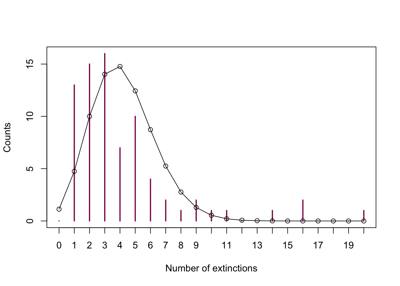
# so, to calculate the expected counts, we need the expected frequencies for 0, 1, 2... extinctions that we can get using dpois and the expected frequency of more than 20 extinction that we get with ppois:
exp = c(dpois(x = 0:19, lambda = mean_ext)*sum(extinctTable),
             (1-ppois(q = 19, lambda = mean_ext))*sum(extinctTable))
Step C: calculate the lack of fit chi^2 statistic (X2obs) of the data to this model
obs = as.vector(extinctTable) # here we are just taking the actual values from our table as a vector

chi_sq = sum(((exp - obs)^2)/exp) #571658
Step D: discuss if /why you should pool some classes, decide on a number of classes and accordingly choose df
We should definitely pool some classes - if we look at the \(chi^2\) value that we obtained, we see that it’s enormous, which is due to the fact that we used the \(chi^2\) test even though our data didn’t meet the assumptions of the test (none of the categories should have an expected count less than 1 and no more than 20% of the categories should have expected counts less than 5).
We can deal with this problem in multiple ways. First, we can create our new vectors “manually”:
obs## [1] 0 13 15 16 7 10 4 2 1 2 1 1 0 0 1 0 2 0 0 0 1new_obs = NULL # we create a null vector
new_obs[1] = obs[1] + obs[2] # we pool together categories 0 and 1
# from category 2 up to 7, nothing changes:
new_obs[2] = obs[3]
new_obs[3] = obs[4]
new_obs[4] = obs[5]
new_obs[5] = obs[6]
new_obs[6] = obs[7]
new_obs[7] = obs[8]
# and then we put everything else to category 8:
new_obs[8] = obs[9] + obs[10] + obs[11] + obs[12] + obs[13] + obs[14] + obs[15]+ obs[16]+ obs[17]+ obs[18]+ obs[19]+ obs[20]+ obs[21]
new_obs## [1] 13 15 16 7 10 4 2 9Alternatively, we can deal with it using a for loop - we loop over our table and every time we see a number that is bigger than 8, we change it to be just 8.
new_obs_loop = NULL

for(i in 1:length(extinctData$numberOfExtinctions)){
  if(extinctData$numberOfExtinctions[i] > 8) {
    new_obs_loop[i] = 8 # changing the values to 8, thus pooling them together
  } else {
    new_obs_loop[i] = extinctData$numberOfExtinctions[i] # we leave the values that are smaller than 8 as they are
  }
}
obs_loop = as.vector(table(new_obs_loop)) # we need the table function so that we don't have just a lot of individual values, but the counts of them
new_exp = c(sum(ppois(q = 1, lambda = mean_ext)*sum(extinctTable)), # the new category having 0 and 1 successes
dpois(x = 2:7, lambda = mean_ext)*sum(extinctTable), # categories having 2 to 7 successes
(1-ppois(q = 7, lambda = mean_ext))*sum(extinctTable)) # 8 or more successesAnd with this, we can obtain the test statistic:
new_chi <- sum(((new_obs - new_exp)^2)/new_exp) #23,95
new_chi_2 <- sum(((obs_loop - new_exp)^2)/new_exp) #23,95
# we get the same chi^2 values with both grouping methods
We can visualize where this \(chi^2\) test statistic value falls:
plot(dchisq(x = 0:25, df = 6), type = "l",
      xlab = "Number of extinctions",
      ylab = "Frequency",
      main = "Chi^2 distribution with 6 degrees of freedom")
abline(v = new_chi, col = "deeppink4") # puts the test statistic value as an abline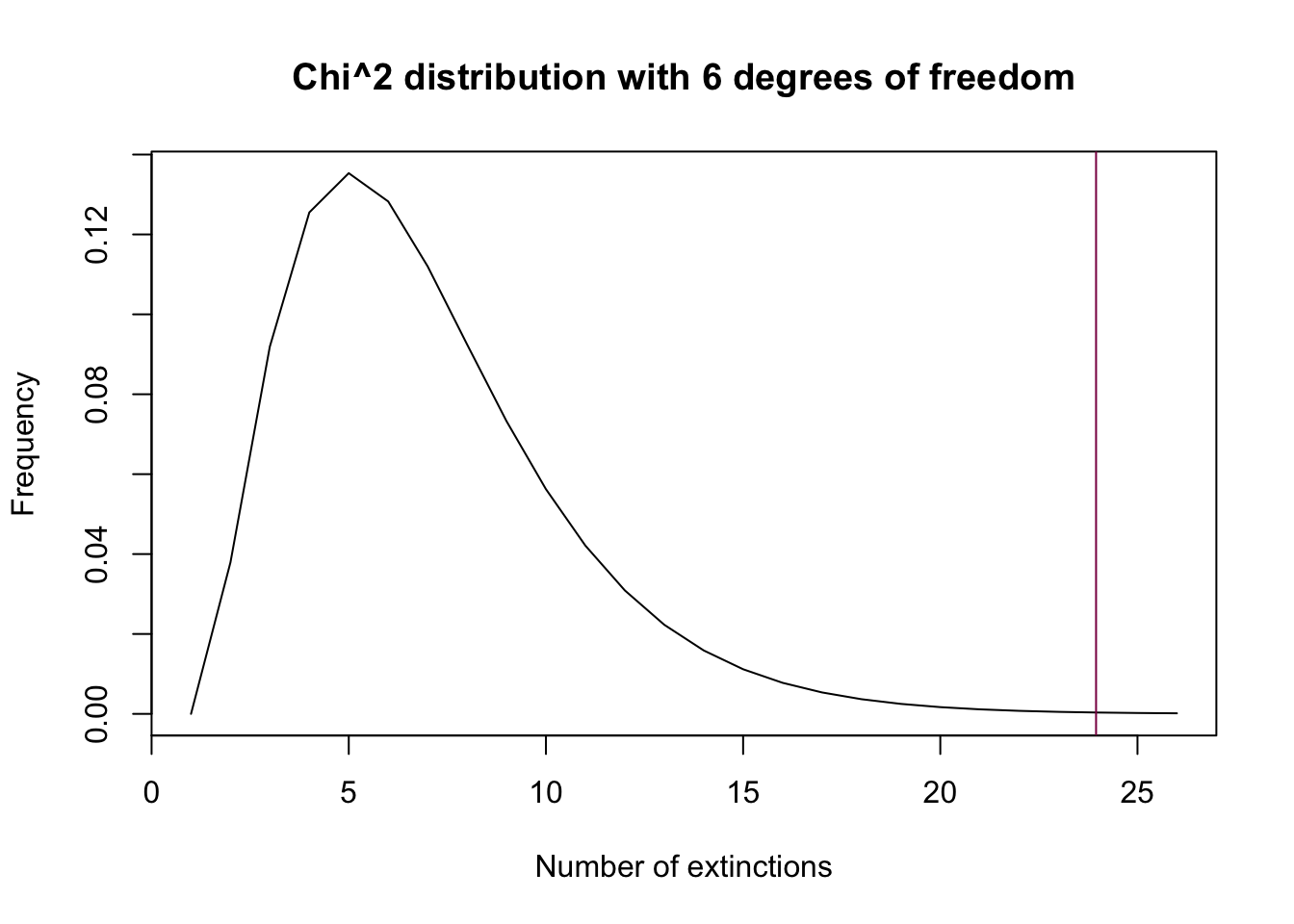
Step E: use pchisq() to get the pvalue: do you accept or reject H0?
1 - pchisq(q = new_chi, df = 6) # we reject the null## [1] 0.0005334919Since the p-value is smaller than 0.01, we reject the null hypothesis - the data is not consistent with the hypothesis that the data is Poisson-distributed.
We can also see if they are dispersed or clumped by comparing the mean to the variance:
var(extinctData$numberOfExtinctions)/mean(extinctData$numberOfExtinctions)## [1] 3.257333Since the variance is larger than the mean, we can say that the extinctions are clumped.
Take me back to the beginning!
Questions from Chapter 8 Problems
At this stage, you have done your warm up in R, and mastered the binomial and \(chi^2\) probability distributions!
Practice Problem 8.1
prog_data = c(rep(0, 118), rep(1, 64), rep(2, 16), rep(3, 2))The Poisson distribution is appropriate in this case because the basic premise of the program is that it places individuals independently and the probability is the same everywhere - and if these indeed hold, then the number of successes per block of space is described by the Poisson-distribution.
\(H_0\): the program places individuals on a spatial landscape randomly \(H_A\): the program doesn’t place individuals randomly (instead, the placement is either dispersed or clumped)
Frequency table of the data:
prog_table = table(prog_data)
prog_table
## prog_data
## 0 1 2 3
## 118 64 16 2- Mean of individuals:
prog_mean = mean(prog_data)
prog_mean
## [1] 0.51- Probability of 0, 1, 2 and 3 individuals per block:
dpois(x = 0, lambda = prog_mean)## [1] 0.6004956dpois(x = 1, lambda = prog_mean)## [1] 0.3062527dpois(x = 2, lambda = prog_mean)## [1] 0.07809445dpois(x = 3, lambda = prog_mean)## [1] 0.01327606- Expected numbers of blocks with 0 to 3 individuals:
prog_exp  = c(dpois(x = 0:2, lambda = prog_mean)*200, # 0, 1 and 2 successes
              (1-ppois(q = 2, lambda = prog_mean))*200) # 3 or more successes
No, they aren’t suitable - more than 20% of the categories have an expected count less than 5. Therefore, we should pool the categories 2 and 3 (or more) together.
Pooling the categories together:
new_prog_obs = NULL

# again, we can do it "manually"
new_prog_obs[1] =  prog_table[1]
new_prog_obs[2] = prog_table[2]
new_prog_obs[3] = prog_table[3] + prog_table[4]

# or with a for loop:
new_obs_loop = NULL

for(i in 1:length(prog_data)){
  if(prog_data[i] > 2){
    new_obs_loop[i] = 2
  }else{
    new_obs_loop[i] = prog_data[i]
  }
}

new_obs_loop_t = as.vector(table(new_obs_loop))

# and then we get the expected counts:
new_prog_exp  = c(dpois(x = 0:1, lambda = prog_mean)*200, # 0 and 1 successes
(1-ppois(q = 1, lambda = prog_mean))*200) # 2 and more successes- We have 3 categories and we calculated the mean, so we have 1 degrees of freedom left.
Degrees of freedom = number of categories - 1 - number of parameters calculated from the data
- \(Chi^2\) test statistic:
prog_chi = sum(((new_prog_obs - new_prog_exp)^2)/new_prog_exp)
prog_chi
## [1] 0.1827849- The p-value:
1 - pchisq(q = prog_chi, df = 1)## [1] 0.6689908- Since the p-value is larger than 0.05, we fail to reject the null hypothesis - the data is consistent with the hypothesis that the program places individuals on a spatial landscape randomly.
Practice Problem 8.2
- Plotting the data:
fish_data = c(rep(0, 103), rep(1, 72), rep(2, 44), rep(3, 14), rep(4, 3), rep(5, 1), rep(6, 1))

hist(fish_data, col = "deeppink4",
     xlab = "Number of nematodes per fish",
     ylab = "Frequency",
     breaks = 7,
     main = "Histogram of the nematode data")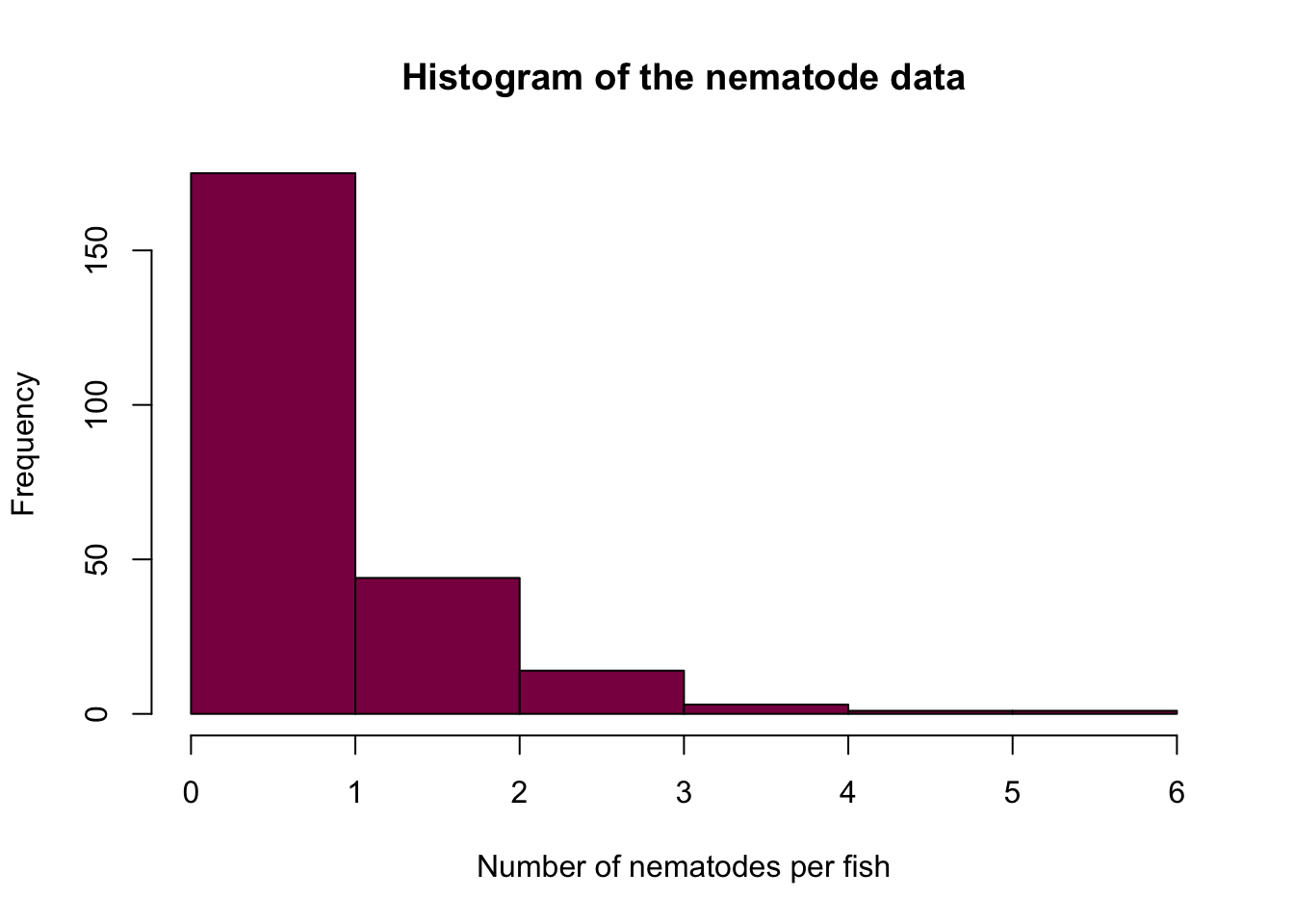
- Expected frequencies:
fish_mean = mean(fish_data)

fish_exp = c(dpois(0:5, lambda = fish_mean),
1-ppois(5, lambda = fish_mean) ) * length(fish_data)- Overlaying the expected frequencies on the graph:
plot(x = 0:6, y = as.vector(table(fish_data)), col = "deeppink4", xlab = "Number of nematodes per fish", ylab = "Frequency", type = "h", lwd = 10)
points(x = 0:6, y =  fish_exp, type = "o")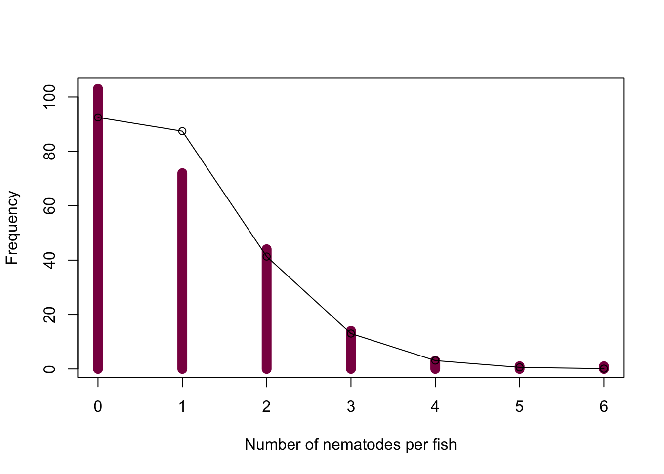
We can see that we observe more fish with 0 nematodes and less fish with 1 nematode than we’d expect under the assumption of randomness, however, the other categories match the expectations well.
- Hypothesis testing:
\(H_0\): Nematodes infect fish at random
\(H_A\): Nematodes do not infect fish at random
fish_table = table(fish_data)

# first, we pool some categories so that the assumptions of the chi^2 test are met - so we have categories 0, 1, 2, 3 and 4 and more
# this is another way to pool - just getting the values from the original data table
fish_obs = c(fish_table[1:4],
             sum(fish_table[5:7]))
fish_exp = c(dpois(0:3, lambda = fish_mean),
             1-ppois(3, lambda = fish_mean))*length(fish_data)

# the test statistic
fish_chi = sum(((fish_obs - fish_exp)^2)/fish_exp)
fish_chi
## [1] 4.570719# the p-value
1 - pchisq(q = fish_chi, df = 3) ## [1] 0.2060684The p-value is bigger than 0.05, so we can’t reject the null hypothesis - nematodes seem to infect fish randomly.
Assignment problem 8.19
- Mean of the number of hurricanes per year:
hurricane_data = c(rep(0, 50), rep(1, 39), rep(2, 7), rep(3, 4))
hurricane_table = table(hurricane_data)

h_mean = mean(hurricane_data)
h_mean
## [1] 0.65If the hurricanes were to hit independently of eachother and if the probability of a hurricane were the same in every year, then the number of hurricanes per year would be described by the Poisson-distribution.
Testing the fit to the Poisson-distribution:
h_exp = c(dpois(x = 0:2, lambda = mean(data)),
          1-ppois(q = 2, lambda = mean(data)))*length(data)
h_obs = as.vector(table(hurricane_data))

h_obs
## [1] 50 39 7 4We need to pool the last 2 categories together.
h_exp_pool = c(dpois(x = 0:1, lambda = h_mean),
               1-ppois(q = 1, lambda = h_mean))*length(hurricane_data)

h_obs_pool = c(hurricane_table[1:2],
               sum(hurricane_table[3:4]))

fish_chi = sum(((h_obs_pool - h_exp_pool)^2)/h_exp_pool)

1 - pchisq(q = fish_chi, df = 1)
## [1] 0.2300109We can’t reject the null hypothesis, hurricanes seem to hit the US randomly through the years.
Take me back to the beginning!
Planning a metagenome sequencing experiment
When you sequence metagenomes you have a soup that consists of say all the bacteria in a water sample. The abundance of the bacteria species can vary a lot in a sample. Here we want to examine how much sequencing we need to do before we can “detect” a rare clade.
We sequence 1kb of the 16S ribosomal DNA (a hypervariable region of this gene is used for doing this). Assume that we have extracted DNA “en masse” from our water sample.
To detect reliably your bacteria you need at least 5 copies of the 16S gene being sequenced. We know that some groups of bacteria make up 50% of these so it is pretty easy to “catch them”.
But what volume of sequencing (expressed in total kb of sequence) do you need to do if you want to have 80% probability to “detect” 1/10 of all bacteria present?
total_vol = 1 # let's start out with the volume of one
bacteria_prop = 0.1 # we want to detect 1/10 of bacteria present

# the easiest way to do this is with a while loop - so we increase the total volume until we see the probability that we calculate with 1-ppois reaching 80% - when it does, the loop terminates and we get the total volume of sequencing we need
while(1-ppois(q = 4, lambda = total_vol*bacteria_prop) < 0.8){
  total_vol = total_vol + 1
}

total_vol
## [1] 68How is your volume of sequencing to be adjusted if you were to detect a group that represents 1/100 (rare) or 1/1000 (super rare) of all bacteria present?
total_vol = 1
bacteria_prop = 0.01

while(1-ppois(q = 4, lambda = total_vol*bacteria_prop) < 0.8){
  total_vol = total_vol + 1
}

total_vol
## [1] 673total_vol = 1
bacteria_prop = 0.001
while(1-ppois(q = 4, lambda = total_vol*bacteria_prop) < 0.8){
total_vol = total_vol + 1
}
total_vol## [1] 6721Take me back to the beginning!