Week 7: Goodness of fit
Wed, Mar 14, 2018 Made by Judit Kisistók, incorporating some snippets from Sara Moeskjær's solution sheet. The exercise session was created by Thomas Bataillon and Palle Villesen at Aarhus University.Learning goals
By the end of this session, you should be able to…
- Understand Goodness-of-fit tests:
- How do we quantify lack of fit for frequency data: the chi2 test stastistic?
- How much lack of fit do we expect “just by chance” under H0?
- The Chi^2 probability distribution and its use as a null distribution for goodness-of-fit tests
- Understand the difference between the Chi^2 statistic and the Chi^2 probability distribution
README FIRST :-) !!!
We first introduce/illustrate THREE important new R functions: dchisq() pchisq() and rchisq().
You then have to apply these functions in a variety of situations.
It’s a good idea to work sequentially:
1. Try the R new functions especially the one that allow you to vizualize and calculate probabilities using the Chi^2 probablity distributions
2. Try the next questions where you will redo in R 2 examples of Chapter 8 step by step
3. Try the set of Chapter 8 practice and assignment problems listed below (also listed in the weekly note)
R functions for simulating from / calculating the Chi^2 probability distribution
If you want to draw 100 random number from a Chi^2 distribution with 1, 2, and 5 degrees of freedom (hereafter d.f):
my100deviates=rchisq(n = 100, df = 1) ## try to evaluate that several times (you get different numbers)
hist(my100deviates, main="100 draws from a Chi^2 1 df", col = "deeppink4")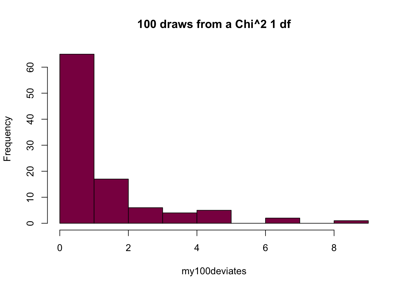
my100deviates=rchisq(n = 100, df = 2) ## try to evaluate that several times (you get different numbers)
hist(my100deviates, main="100 draws from a Chi^2 2 df", col = "deeppink4")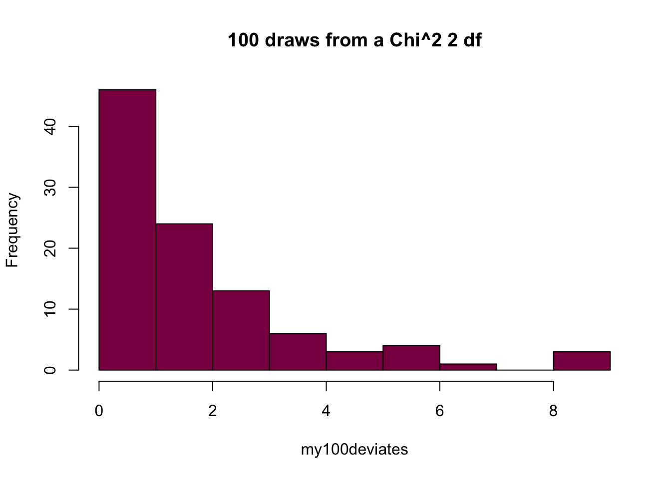
my100deviates=rchisq(n = 100, df = 5) ## try to evaluate that several times (you get different numbers)
hist(my100deviates, main="100 draws from a Chi^2 5 df", col = "deeppink4")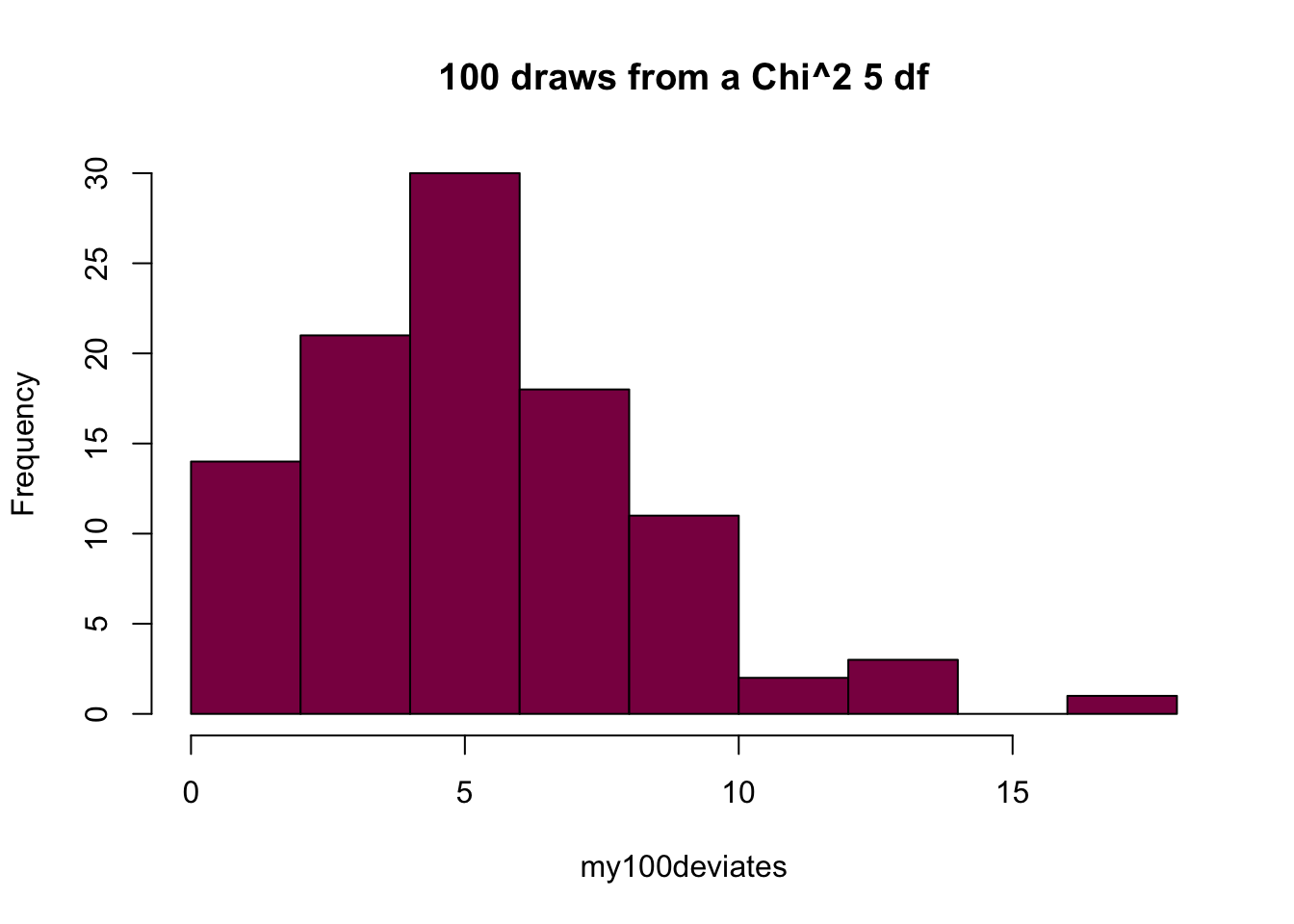
If you want to graph the Chi^2 probability distribution: you have to “plot” the density function over a grid of coordinates
xs= seq(from = 0.01, to=10, by=0.05 ) # xs is a vector of coordinates on the X axis

y1=dchisq(x =xs , df = 1) #y1 stores the density of the Chi^2 (1 d.f) distribution at each coordinate.

y2=dchisq(x =xs , df = 2) #y2 stores the density of the Chi^2 (2 d.f) distribution at each coordinate.

y6=dchisq(x =xs , df = 6) #y6 stores the density of the Chi^2 (6 d.f) distribution at each coordinate.
Visualizing Chi^2 distributions in R: Plotting the densities of 3 different Chi^2 distributions
plot(xs,y1, type ="l", lwd=3)  # Plotting the density of the Chi^2 (1.df) probability distribution

lines(xs,y2, type ="l", lwd=3, col="blue")  #Adding the density of the Chi^2 (1.df) probability distribution, on the previous plot

lines(xs,y6, type="l", lwd=3, col="magenta")#Adding the density of the Chi^2 (1.df) probability distribution, on the previous plot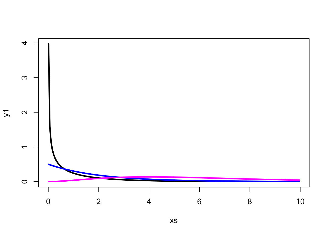
If you want to calculate the area under the curve of the density of a Chi^2 distribution you need to do an integral and pchisq() can do that:
pchisq(q = 10,df = 1) # This calculates P( X <10) if X is a random variable following a Chi^2 (1 d.f) probability distribution## [1] 0.9984346pchisq(q = 10,df = 6) # This calculates P( X <10) if X is a random variable following a Chi^2 (1 d.f) probability distribution## [1] 0.875348plot(xs,y1, type ="l", lwd=3, ylim=c(0,2)) # we need to choose the range of Y wisely to be able to plot these distributions properly
lines(xs,y2, type ="l", lwd=3, col="blue") #Adding the density curve of the Chi^2 (1.df) probability distribution, on the previous plot
lines(xs,y6, type="l", lwd=3, col="magenta")#Adding the density curve of the Chi^2 (1.df) probability distribution, on the previous plot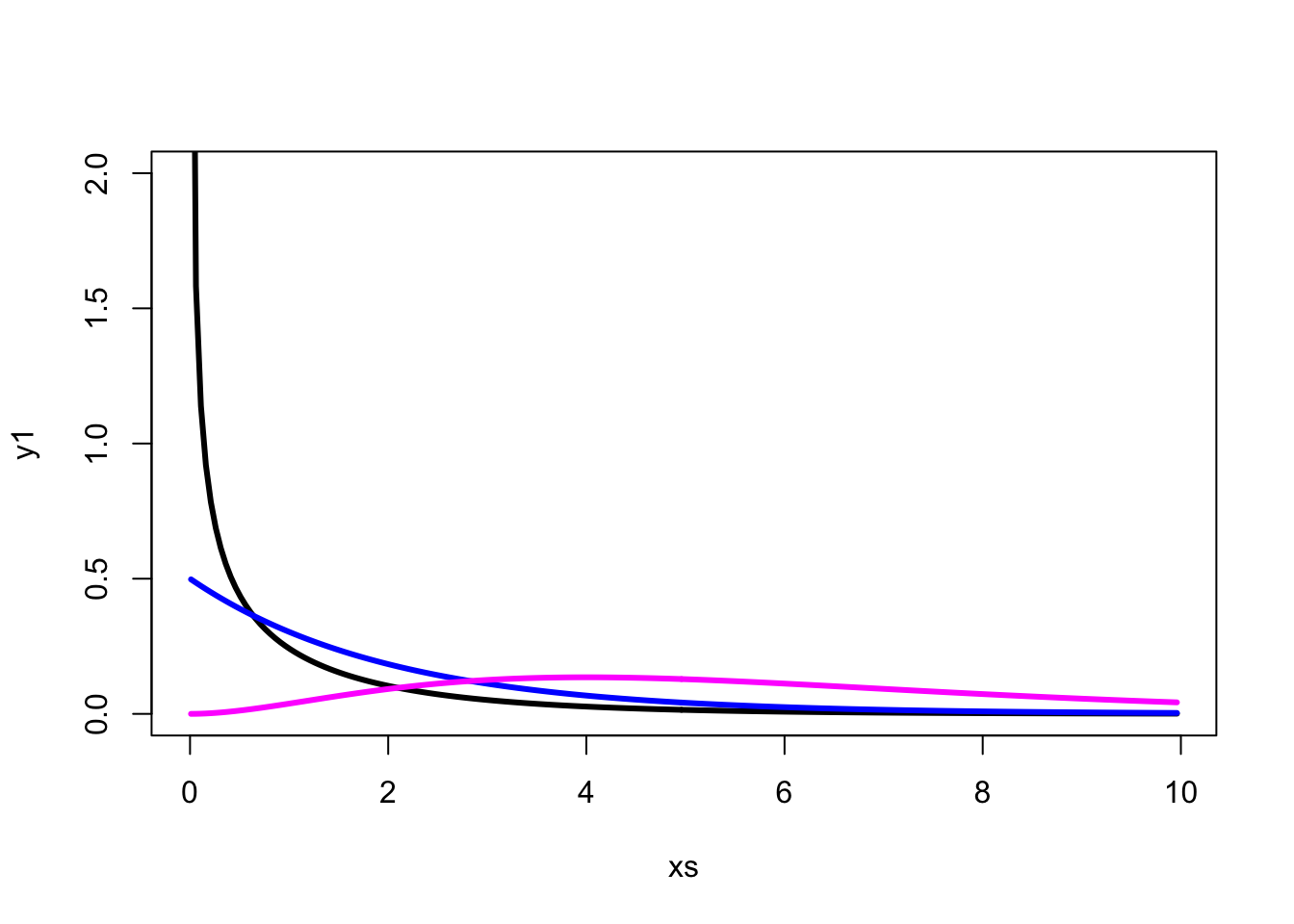
Take me back to the beginning!
Mastering Chi^2 distributions using dchisq(), pchisq() and rchisq()
Let’s call:
- XX1 a random variable that follows a probability distribution that is Chi^2 (1 d.f)
XX1 = rchisq(n = 1, df = 1)- XX6 a random variable that follows a distribution that is Chi^2 (6 d.f)
XX6 = rchisq(n = 1, df = 6)Note that we just drew 2 numbers from the corresponding chi^2 distributions.
Generate 10^5 draws from the distributions of XX1 and XX6 use these draws to calculate:
P(1 < XX1 < 2)
P(XX6 > 25)
# simulating the distribution
XX1_distr = rchisq(n = 10^5, df = 1)
# calculating the p-value by summing up how many times to I see a number in my simulated distribution that's between 1 and 2, and dividing it by the number of simulated values (10^5)
p_XX1_s = length(XX1_distr[XX1_distr > 1 & XX1_distr < 2]) / length(XX1_distr)

# and then we can plot it
hist(XX1_distr, col = "deeppink4", xlim = c(0,10), breaks = 100)
# and put our XX1 random variable on the plot to see where it is in the distribution
abline(v = XX1)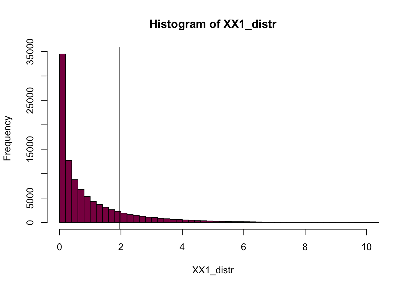
# same thing with XX6
XX6_distr = rchisq(n = 10^5, df = 6)
p_XX6_s = length(XX6_distr[XX6_distr > 25]) / length(XX6_distr)

hist(XX6_distr, col = "deeppink4", xlim = c(0,10), breaks = 100)
abline(v = XX6)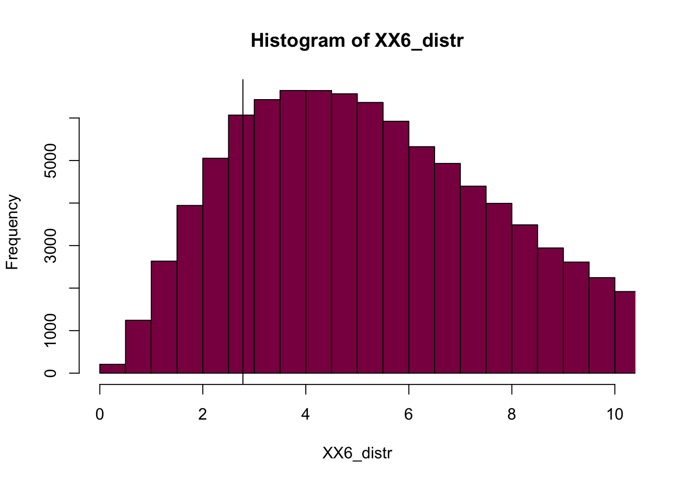
Use pchisq() to calculate cand compare with your simulation based results.
P( 1 < XX1 < 2)
P( XX6 > 25)
pchisq(q = 2,df = 1) # P(X < 2)## [1] 0.8427008pchisq(q = 1,df = 1) # P(X < 1)## [1] 0.6826895# to get the "middle part", aka the part between 1 and 2, we need to calculate the probability that X is smaller than 2 and divide the probability that X is smaller than 1
p_XX1_r = pchisq(q = 2,df = 1) - pchisq(q = 1,df = 1)
p_XX6_r = 1-pchisq(q = 25,df = 6)Using qchisq() calculate the probabilities below:
Find the critical values C, such that - P(X1 < C) = 0.95
- P(X1 > C) = 0.01
- P(X6 > C) = 0.01
# P(XX1 < C) = 0.95
qchisq(0.95, df=1)
## [1] 3.841459# P(XX1 > C) = 0.01
qchisq(0.01, df=1)## [1] 0.0001570879# P(XX6 > C) = 0.01
qchisq(0.01, df=6)## [1] 0.8720903Calculate critical values for the 5% level of a Chi^2 with 1, 2 and 6 d.f. Visualize the three densities and their critical values on the graph using the rug() function, or use the abline(v= C) to set a vertical line at the C coordinate.
xs= seq(from = 0.01, to=13, by=0.05 )
y1=dchisq(x =xs, df = 1)
y2=dchisq(x =xs, df = 2)
y6=dchisq(x =xs, df = 6)

plot(xs,y1, type ="l", lwd=3, ylim=c(0,2), col = "coral", xlim = c(0,13))
lines(xs,y2, type ="l", lwd=3, col="skyblue")
lines(xs,y6, type="l", lwd=3, col="seagreen3")
abline(v = qchisq(0.95, df=1), col = "coral")
abline(v = qchisq(0.95, df=2), col="skyblue")
abline(v = qchisq(0.95, df=6), col="seagreen3")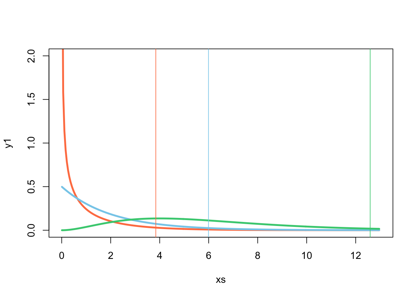
Take me back to the beginning!
No weekend getaway (Example 8.1 from the book)
Reproduce in R the calculations of the example: - calculate the lack of fit “chi square” statistic X2obs
- use pchisq() to get the p-value
expected = NULL
expected[1:5] = 350*(52/365)
expected[6] = 350*(53/365)
expected[7] = 350*(52/365)

observed = c(33, 41, 63, 63, 47, 56, 47)

weekend_data <- as.data.frame(cbind(expected, observed)) #putting it all to a dataframe in case we want to look at it later
# and it's also useful to have for plotting purposes
rownames(weekend_data) <- c("Sun", "Mon", "Tue", "Wed", "Thu", "Fri", "Sat")

# this gives a barplot - t() stands for transpose, it basically turns the columns into rows to help R draw the graphs properly
barplot(t(weekend_data), beside = TRUE, col=c("deeppink4","lightblue"), legend = colnames(weekend_data))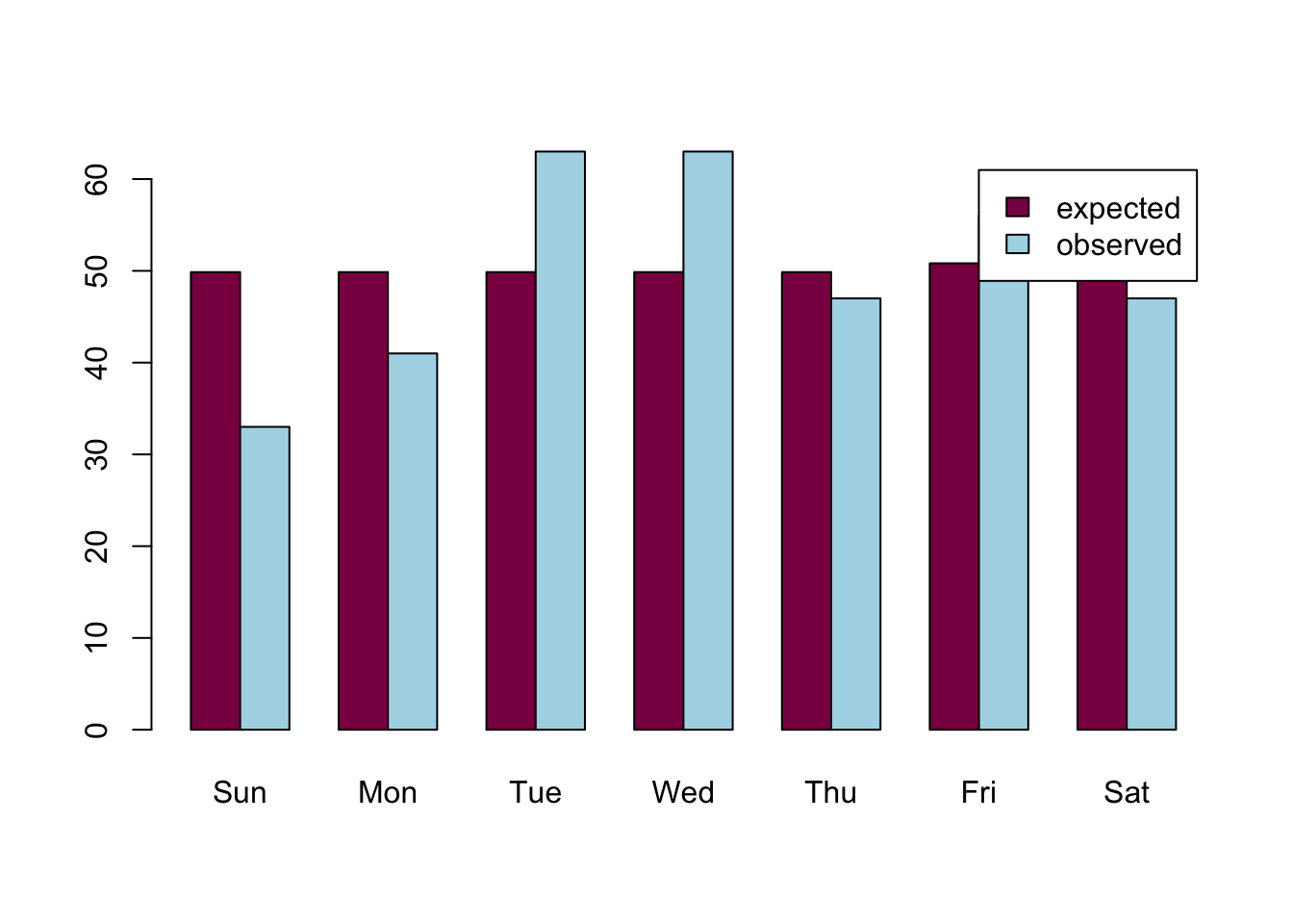
X2obs = sum((observed-expected)^2/expected) # the chi^2 statistic
# here we are doing calculations with vectors - what R is doing is that it goes through the vectors simultaneously, element by element, and does the operations like that - so first, it takes the first element from the observed vector and the first element from the expected vector, does the calculations, then moves on to the second elements and so on, and at the end it sums them up, giving us the chi^2 value

p_value1 <- 1 - pchisq(q = X2obs, df = 6)
# a little bit different way to get the p-value - if you specify lower.tail = FALSE, you get P[X > X2obs]
p_value2 <- pchisq(q = X2obs, df = 6, lower.tail=FALSE)
Take me back to the beginning!
Gene content of the human X chromosome (Example 8.4 from the book)
H0: 5.2% of genes in the human genome are located on the X (this is an a priori expectation based on physical size of the X)
Calculate in R the test statistic that quantifies the lack of fit between observed and expected counts (we call that X2obs)
n = 20290
expectedX = c(1055, 19235)

observedX = c(781, 19509)

X2obsX = sum((observedX-expectedX)^2/expectedX)
Calculate the p-value for a goodness of fit test assuming that under H0 X2obs should be Chi^2 with 1.df
1-pchisq(q = X2obsX, df = 1)## [1] 0# there are significantly less genes on the X than we would expectWhy is the p value for this case NOT calculated as 2* Pr(X1 > X2obs…) ?
X^2 approaching 0 actually means that we have a good fit - and every deviation is going to increase the value of X^2. Therefore, in this context, only the upper tail is meaningful in terms of calculating the p-value.
Do a binomial test as way to do a goodness of fit and calculate p-value using the binomial distribution
2*pbinom(q = 781, size = 20290, prob = 0.052) # this is how you calculate it using pbinom## [1] 1.507498e-19sum(dbinom(x = 0:781, size = 20290, prob = 0.052)*2) # and this is how to do it with dbinom## [1] 1.507498e-19Take me back to the beginning!
Designer 2 child families (Example 8.5 from the book)
Redo in R the different steps of goodness of fit test to test the hypothesis that the data presented in table 8.5-1 is binomial
data = read.csv("chap08e5NumberOfBoys.csv")

total_nr = nrow(data) #2444 families

boy_0_obs = length(data[data == 0]) #530
boy_1_obs = length(data[data == 1]) #1332
boy_2_obs = length(data[data == 2]) #582

# we estimate the proportion of boys
prop = (boy_1_obs + 2*boy_2_obs) / (2*total_nr)

boy_0 = dbinom(x = 0, size = 2, prob = prop)
boy_0_exp = boy_0 * total_nr #expected number of families with 0 boys

boy_1 = dbinom(x = 1, size = 2, prob = prop)
boy_1_exp = boy_1 * total_nr #expected number of families with 1 boy

boy_2 = dbinom(x = 2, size = 2, prob = prop)
boy_2_exp = boy_2 * total_nr #expected number of families with 0 boys

#plot the data and see how the observed and expected frequencies differ
boy_data = as.data.frame(cbind(rbind(boy_0_obs, boy_1_obs, boy_2_obs), rbind(boy_0_exp, boy_1_exp, boy_2_exp))) # putting every counts into the same dataframe
# rbind creates the rows (row-bind) and cbind creates the columns (column-bind)

rownames(boy_data) <- c("0 boys", "1 boy", "2 boys")

colnames(boy_data) <- c("Observed", "Expected") #naming the columns in the matrix
barplot(t(boy_data), beside = TRUE, col=c("deeppink4","lightblue"), legend = colnames(boy_data))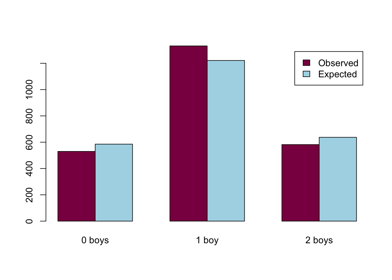
# calculating chi square
chi_sq = sum(((boy_data$Observed - boy_data$Expected)^2) / boy_data$Expected)

# degrees of freedom & calculating the critical value
df = 1 #3 categories, and we had to estimate prop from the data

chi_krit = qchisq(0.05, df=1) #critical value at the 0.01 significance level - 0.0039

chi_sq < chi_krit #FALSE - we reject the null
## [1] FALSETake me back to the beginning!
Questions from Chapter 8 Problems
At this stage, you have done your warm up in R, and mastered the binomial and Chi^2 probability distributions! In Chapter 8 do: Practice problem 3, Practice problem 5 (skip 5.d), Practice problem 6, Assignment Problem 12+13 - calculate them manually and in R as well.
You can find the answers to Practice problem 3, 5 and 6 in the book. Here is Assignment problem 12 to walk you through a goodness of fit test again:
# the data
number_of_bears = 87
BB_count = 42
Bb_count = 24
bb_count = 21

# H0: the frequency of b alleles follows a binomial distribution
# HA: it doesn't

# fraction of b alleles in the population:
p_b = (1*24 + 2*21) / (2*87) #0,379

# expected frequency of bears with 0, 1 and 2 b alleles
b_0 = dbinom(x = 0, size = 2, prob = p_b)
b_0_exp = b_0*number_of_bears #expected number of bears with 0 b alleles: 33,5

b_1 = dbinom(x = 1, size = 2, prob = p_b)
b_1_exp = b_1*number_of_bears #expected number of bears with 1 b allele: 41

b_2 = dbinom(x = 2, size = 2, prob = p_b)
b_2_exp = b_2*number_of_bears #expected number of bears with 2 b alleles: 12,5

#plot the data and see how the observed and expected frequencies differ
bear_data = as.data.frame(cbind(rbind(BB_count, Bb_count, bb_count), rbind(b_0_exp, b_1_exp, b_2_exp))) #putting every count into the same dataframe

colnames(bear_data) <- c("Observed", "Expected") #naming the columns in the matrix
barplot(t(bear_data), beside = TRUE, col=c("deeppink4","lightblue"), legend = colnames(bear_data))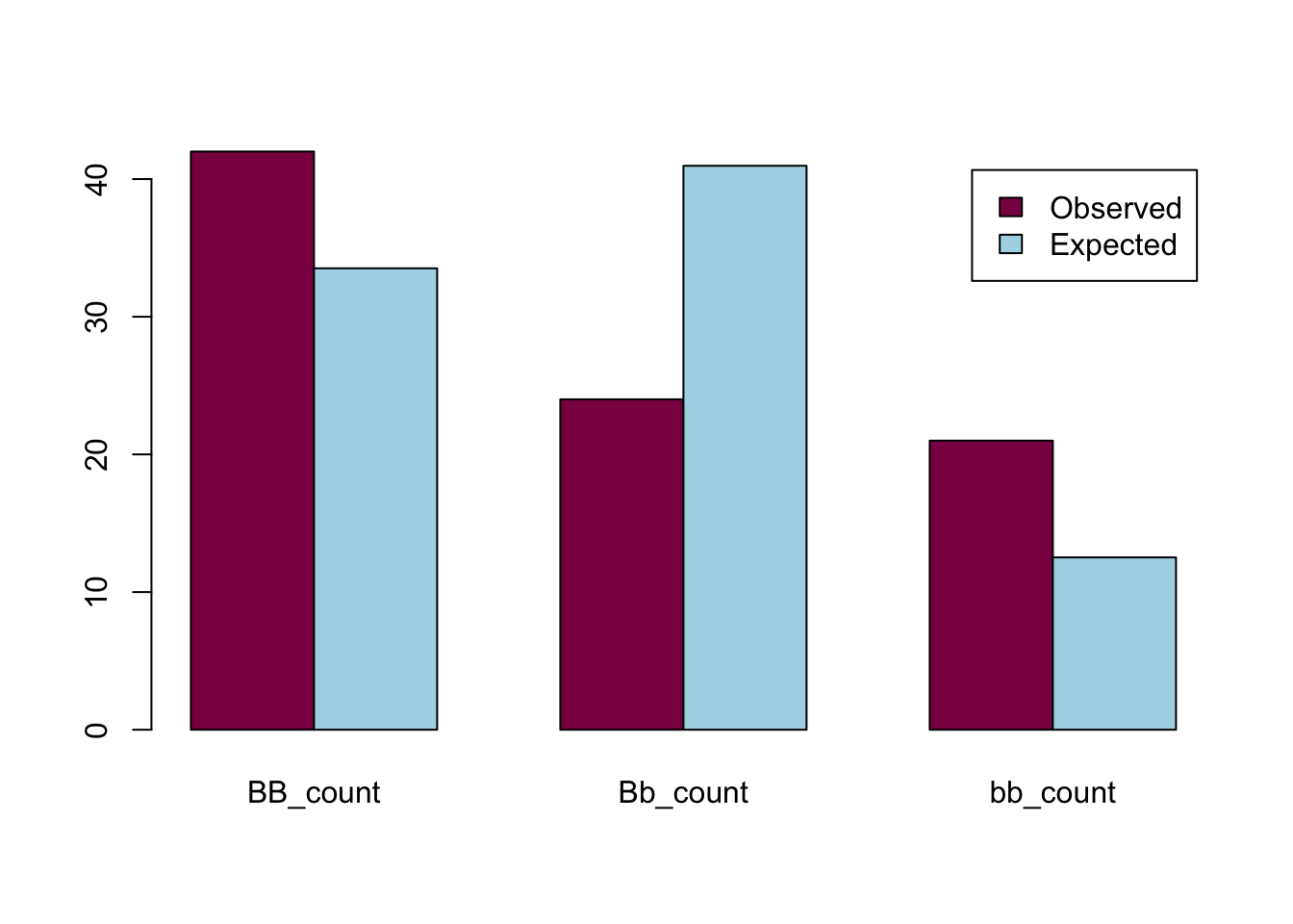
# calculating chi square
chi_sq = sum(((bear_data$Observed - bear_data$Expected)^2) / bear_data$Expected) #14.92

# degrees of freedom & calculating the critical value
df = 1 #3 categories, and we had to estimate p_b from the data

chi_krit = qchisq(0.05, df=1) #critical value at the 0.01 significance level - 0.0039

chi_sq < chi_krit #FALSE - we reject the null
## [1] FALSE