By the end of this session, you should be able to…

• Understand conditional probability
• Understand Bayes theorem: how to calculate the conditional probability
• Understand several key concepts within hypothesis testing
  • Null hypothesis
  • Null distribution
  • Test statistic
  • P value (probability of observing the value of the test statistic if the null hypothesis were true)

What does the sample() function do?

It’s going to shuffle your data around and resample with or without replacement (depending on whether you write replace = TRUE or replace = FALSE).

You can use this to simulate a die:

sample((1:6), size=1,replace=TRUE)

## [1] 6

Or a coin:

sample(c("plat","krone"), size=1, replace=TRUE)

## [1] "krone"

Or just shuffle data around:

sample(1:100)

##   [1]  32  79  28  72  29  27  97  94  67  63  50  96  78 100  19  35  37
##  [18]  17  55  61  89  43  26  16  90  20  23  71  73   1  18  34  15  39
##  [35]  21  46  22  31  24   2  64  95   9  93  83  62  36  98  56   6  30
##  [52]  13  53   4  14  88  76  66  84  38  40  77  48  12  85   7  81  25
##  [69]  42  87  59   8  65  70  60  54  80  44  91  75  33  58  10  45  68
##  [86]  11  51  99  47  41   3  49  69  74   5  57  52  82  92  86

What does set.seed() do?

set.seed(0)
sample(x = c("L", "R"), size = 18, replace = TRUE, prob = c(0.5,0.5) )

##  [1] "L" "R" "R" "L" "L" "R" "L" "L" "L" "L" "R" "R" "R" "L" "R" "L" "R"
## [18] "L"

set.seed(0)
sample(x = c("L", "R"), size = 18, replace = TRUE, prob = c(0.5,0.5) )

##  [1] "L" "R" "R" "L" "L" "R" "L" "L" "L" "L" "R" "R" "R" "L" "R" "L" "R"
## [18] "L"

set.seed(0)
sample(x = c("L", "R"), size = 18, replace = TRUE, prob = c(0.5,0.5) )

##  [1] "L" "R" "R" "L" "L" "R" "L" "L" "L" "L" "R" "R" "R" "L" "R" "L" "R"
## [18] "L"

Sampling is inherently random - setting the seed will cause the sampling to give the same result every time (given every other parameter is the same), making your “experiment” reproducible.

An example of summarising a sample:

x = sample(x = c("A", "B"), size = 1000, replace = TRUE, prob = c(0.5,0.5) )
sum(x=="B") # means that there are this many B's in your sample

## [1] 517

Notice that when you say x = c(“A”, “B”), you essentially define x to be these 2 values. Then, when you re-define x to be a sample of size 1000 taken from these 2 values, what you do is you pick a value, you “write it down”, then you put it back (because you said replace = TRUE) and repeat this 1000 times.

What about sampling without replacement? In that case, you have one less datapoint after every round because after you pick a value and write it down, you put it away. Try running this code after setting replace = FALSE - it will throw an error, because you can’t take 1000 samples from something that has only 2 elements as you run out of things to sample after the second round.

How many “A” in this large sample of 1000 observations?

set.seed(47)
x = sample(x = c("A", "B", "O"), size = 1000, replace = TRUE)
sum(x=="A")

## [1] 324

Example of a simulation:

set.seed(0)
nl = rep(NA,100) # creates a vector of length 100, consisting of NAs (Not Available - used in the case of missing data)
for (i in (1:length(nl))) { #you want to populate the nl vector, hence you want to run this loop as many times as long the nl vector is
  x = sample(x = c("A", "B", "O"), size = 10, replace = TRUE) # you take the sample
  nl[i] = sum(x=="A") # you calculate how many A's are there in that sample and put it in the i-th position in the nl vector
  # rinse and repeat
}

x

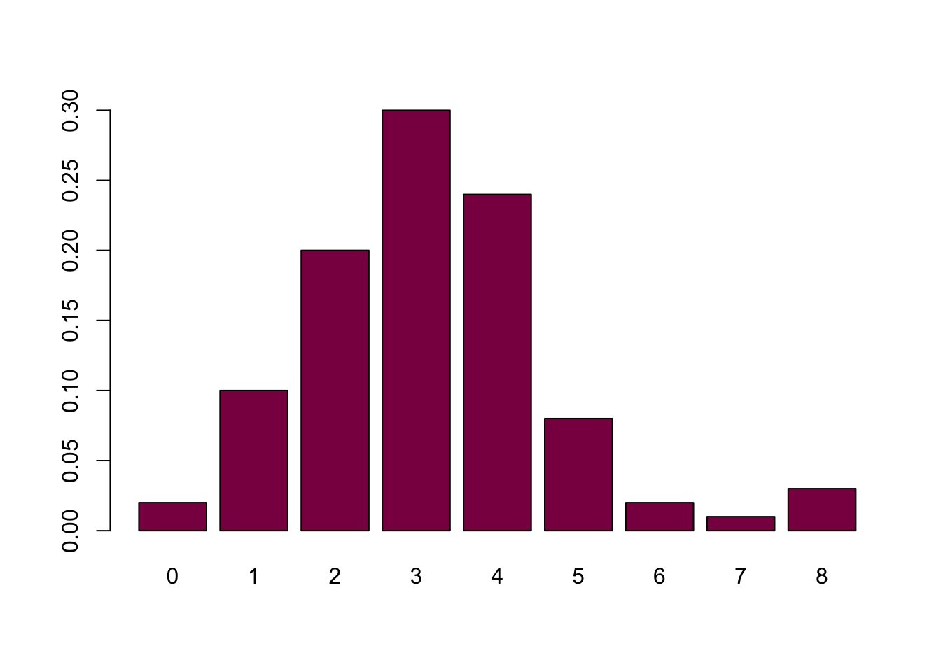
##  [1] "B" "A" "B" "B" "A" "A" "O" "B" "A" "A"

Summary (and the frequency distribution of A’s):

table(nl) # how many times do you see 0...8 A's 

## nl
##  0  1  2  3  4  5  6  7  8 
##  2 10 20 30 24  8  2  1  3

table(nl)/length(nl) # same idea, but with fractions

## nl
##    0    1    2    3    4    5    6    7    8 
## 0.02 0.10 0.20 0.30 0.24 0.08 0.02 0.01 0.03

barplot(table(nl), col = "deeppink4") # histogram visualizing the counts (absolute frequencies)

barplot(table(nl)/length(nl), col = "deeppink4") # histogram visualizing the fractions - same tendencies, different scale (relative frequencies)

Counting extreme values:

sum(nl >= 8)

## [1] 3

sum(nl >= 8) / length(nl)

## [1] 0.03

sum(nl <= 2)

## [1] 32

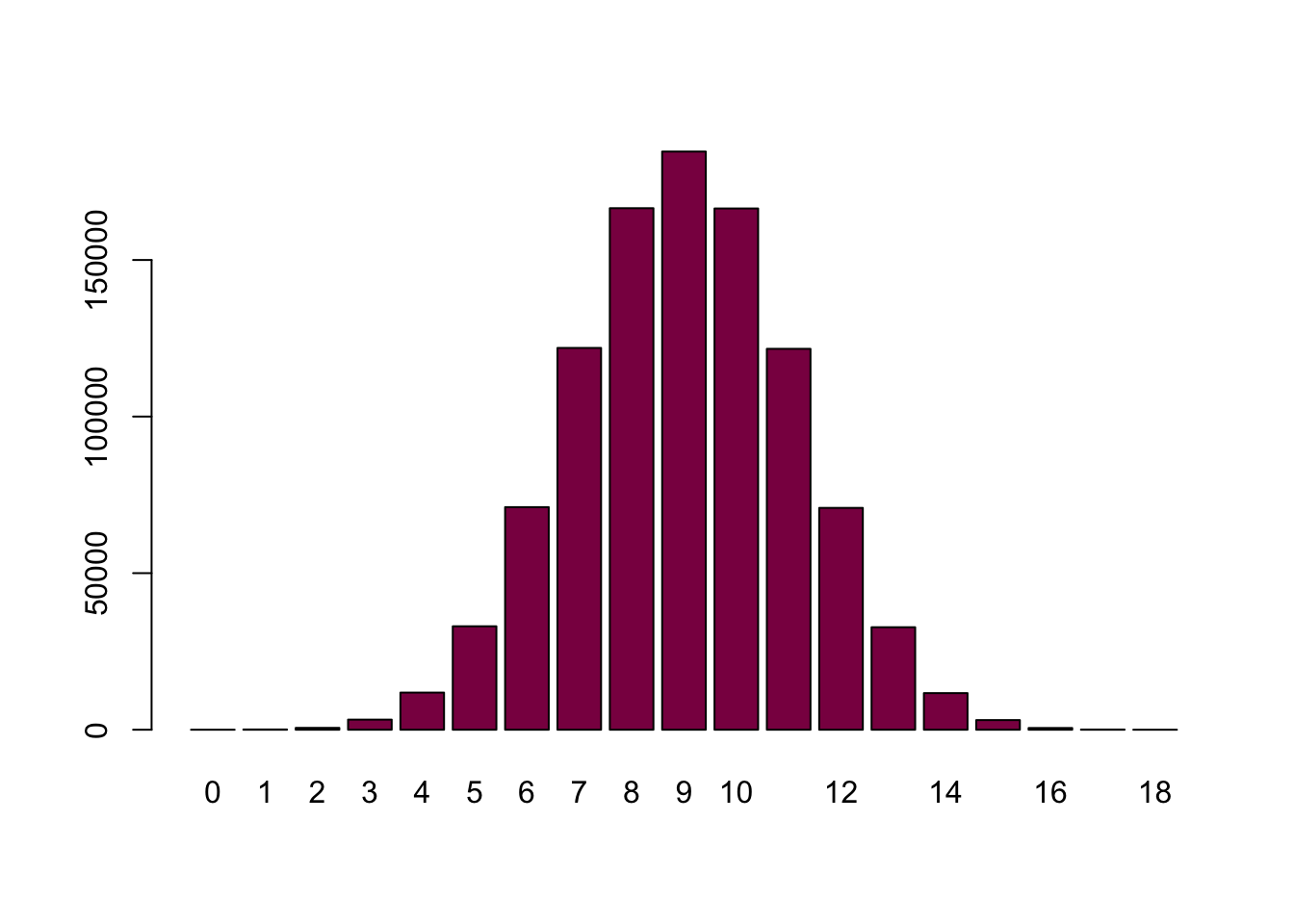
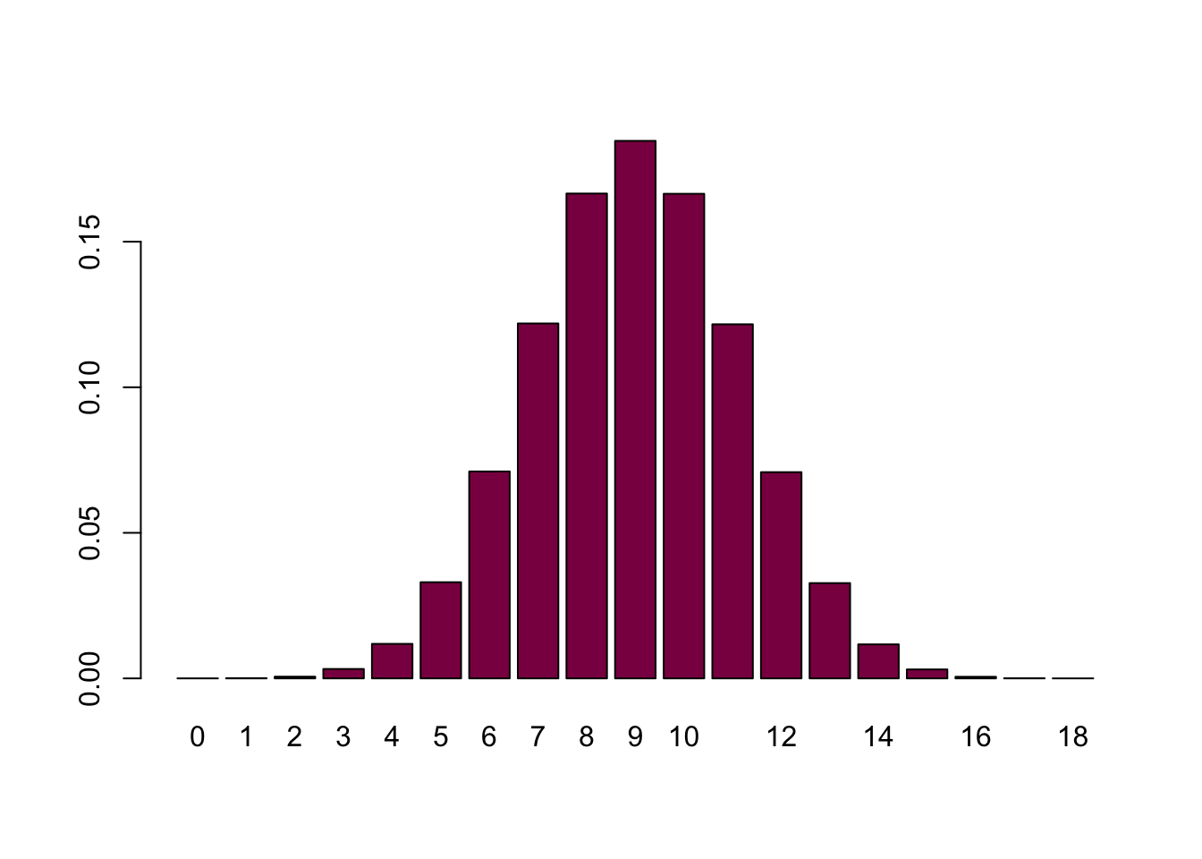
Use the information above to simulate 1 million random samples of 18 toads and make the barplot. We assume that the probability of left is 0.5 and right is 0.5 (null hypothesis).

set.seed(0)
nl = rep(NA,1000000)

for (i in (1:length(nl))) {
  x = sample(x = c("L", "R"), size = 18, replace = TRUE, prob = c(0.5,0.5) )
  nl[i] = sum(x=="L")
}

barplot(table(nl), col = "deeppink4")

barplot(table(nl)/length(nl), col = "deeppink4")

Compare you table of frequencies of left handed toads with table 6.2-1.

table(nl)/length(nl)

## nl
##        0        1        2        3        4        5        6        7 
## 0.000008 0.000080 0.000590 0.003229 0.011858 0.033034 0.071079 0.121916 
##        8        9       10       11       12       13       14       15 
## 0.166540 0.184632 0.166451 0.121632 0.070837 0.032731 0.011689 0.003080 
##       16       17       18 
## 0.000552 0.000060 0.000002

It may not be the same for the very rare outcomes - why?

It’s because if something has a very small probability, you need to take a lot of samples to observe it at least once. For example, if something has 1% probability, you’ll need to try approximately 100 times until you observe it once.

Take me back to the beginning!

Calculate the probability of all 18 toads to be left handed.

0.5^18

## [1] 3.814697e-06

Individually, every toad has 50% chance to be left-handed, so you just multiply this 18 times. This statement is essentially: Pr[first toad is left-handed AND … AND 18th toad is left-handed].

You can, of course, calculate this probability from your simulated distribution - but beware, it won’t give you the same exact result due to the fact that simulations introduce a whole lot of randomness. The answer above is grounded in maths and theory, the answer you’d get from the distribution is grounded in (simulated) data.

Calculate the probability of all 18 toads to be left handed.

0.5^18

## [1] 3.814697e-06

Calculate the probability of 17/18 toads to be left handed (it is 18 different outcomes).

18*(0.5^17*0.5)

## [1] 6.866455e-05

This statement is saying the following: Pr[first toad is left-handed AND … AND 17th toad is left-handed AND 18th toad is right-handed], so to deal with the left-handed ones, you multiply 0.5 17 times and then you multiply this by 0.5 to account for the one right-handed toad. Because you can choose that one right-handed toad in 18 different ways (aka any toad out of the 18 could be the right-handed one), you need to multiply this whole expression by 18.

Calculate the probability of all 18 toads to be left handed if we expect the population to have a frequency of 30% “left handed” toads.

0.3^18 

## [1] 3.874205e-10

Calculate the probability of all 18 toads to be right handed if we expect the population to have a frequency of 30% “left handed” toads.

0.7^18 # because the probability of being right-handed now is 0.7

## [1] 0.001628414

Let’s calculate the probability of 17/18 toads to be left handed if we expect the population to have a frequency of 30% “left-handed” toads now and see how the expression changes:

18*(0.3^17*0.7)

## [1] 1.627166e-08

We can see that this is a much smaller probability, which makes sense as right-handed toads are more than twice as frequent in the population - so we wouldn’t be suprised if it was pretty hard to take a sample where an overwhelming majority (almost 95%) of the toads are left-handed.

Take me back to the beginning!

How often did your simulation yield 14 or more left handed toads?

sum(nl >= 14)

## [1] 15383

How often did it yield the equivalent “lower tail”? (i.e. a similar lower than expected number of left handed toads)

sum(nl <= 4)

## [1] 15765

What is the sum of extreme simulations from the null distribution?

sum(nl >= 14) + sum(nl <= 4)

## [1] 31148

How much is this sum out of the total number of simulations?

(sum(nl >= 14) + sum(nl <= 4)) / length(nl)

## [1] 0.031148

How does this value compare with the obtained P value from the book example?

It is the same value, however, it is based on simulations and not real probabilities.

If you only observed 13 left handed toads - would you reject the null hypothesis?

(sum(nl >= 13) + sum(nl <= 5)) / length(nl)

## [1] 0.096913

We wouldn’t.