Week 1: Introduction
Wed, Jan 31, 2018 Made by Judit Kisist??k. The R exercise session was created by Palle Villesen and Thomas Bataillon at Aarhus University.Learning goals
By the end of this session, you should be able to…
- Open an existing R script
- Save an existing R script
- Create a new R script
- Know the 4 panels in RStudio
- Know how and where to get help (StackOverflow, Google Groups)
1. The basics of R
Whenever you need to use a package, you might need to install it first (without the #) - this only needs to be done once:
#install.packages("binom")But installing is not enough - everytime you want to use this package, you need to load it like this:
library(binom) #notice that you don't need the quotation marks anymoreThis operation will fail if the package is not installed. If the package is installed, you can also click on Packages in the lower right panel of RStudio, look for the one you need and put a checkmark in the checkbox - this will also load it for you.
You might want to clear the console - for that, use the Edit menu or the keyboard shortcut (ctrl-L on Windows and ctrl-l on Mac).
If you want to restart R, use the Session menu or the keyboard shortcut ctrl + shift + f10 (Windows) / shift + cmd + f10 (Mac).
You can get help using “?”
?library
help(library)
You can load a dataset like this:
birdAbundanceData = read.csv("chap02e2bDesertBirdAbundance.csv")CSV stands for comma separated values, so this command will be useful if you have such data. To see how you can import other types of data, check out the Data Import Cheat Sheet on this page.
You can get information about a dataset using the summary() function, including the variables, the smallest and largest values you have and some summary statistics - you can see the mean and the median, and you can even calculate the interquartile range from the 3rd and 1st quartile the summary shows you:
summary(birdAbundanceData)## species abundance
## American Kestrel : 1 Min. : 1.00
## Ash-throated Flycatcher: 1 1st Qu.: 3.50
## Bell's Vireo : 1 Median : 18.00
## Black Vulture : 1 Mean : 74.77
## Black-chin. Hummingbird: 1 3rd Qu.:102.50
## Black-tail. Gnatcatcher: 1 Max. :625.00
## (Other) :37Take me back to the beginning!
2. Plotting
This is how you make a histogram:
# first, we generate some data
mydata = data.frame(var = "label", count = c(1,1,1,3,3,7,7,9,9,1,1,2,2,2,2))
mydata
## var count
## 1 label 1
## 2 label 1
## 3 label 1
## 4 label 3
## 5 label 3
## 6 label 7
## 7 label 7
## 8 label 9
## 9 label 9
## 10 label 1
## 11 label 1
## 12 label 2
## 13 label 2
## 14 label 2
## 15 label 2hist(mydata$count, breaks=20)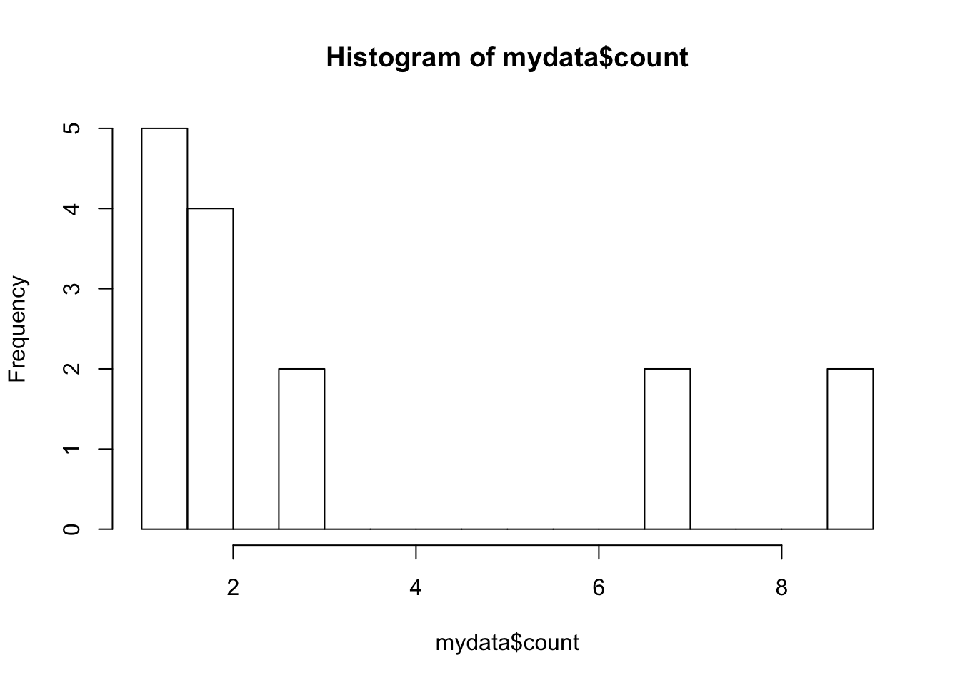
When you make a histogram (and a gazillion other operations in R), you need to specify which column (variable) you want to use from your data, as there is often a lot of them - you can use the $ for that.
Generally, mydata$counts means that “dear R, please take mydata, do something with the variable that’s called ‘counts’, and ignore the rest for now”.
Make a histogram like Figure 2.2-3:
hist(birdAbundanceData$abundance, breaks = 20)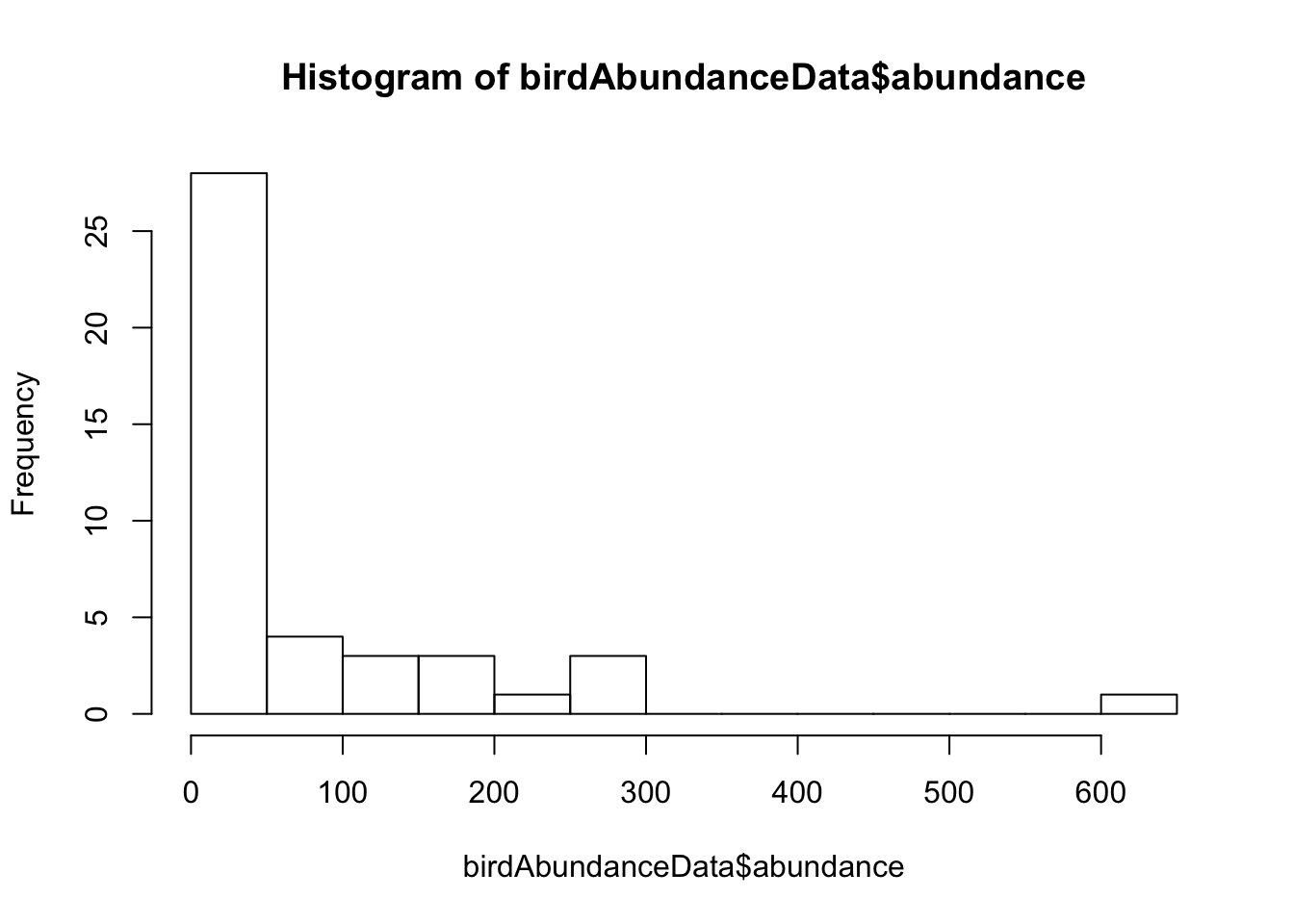
Of course, we can make it fancier:
hist(birdAbundanceData$abundance, breaks = 20, col = "deeppink4", main = "Histogram of bird abundance data", xlab = "Abundance")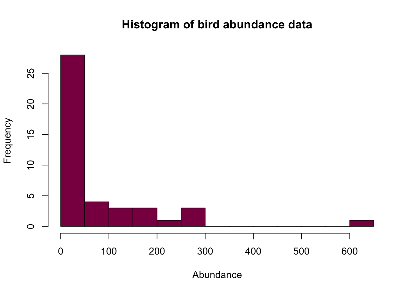
- col: color of the histogram
- main: title
- xlab: label on the X axis
- breaks: you can control the bins with this (whether you want wider or more fine-grained ones) - however, the number you put in doesn’t necessarily correspond to the exact number of bins on the histogram. This is because of the way R runs its algorithm to break up the data but you get something that’s pretty close to what you wanted. Also, there are no strict rules about the number you should use for the breaks - always look at the data and see what makes sense in that context.
You can go to the book homepage and try the R code you can find there.
Histogram for a numeric variable:
hist(birdAbundanceData$abundance, right = FALSE)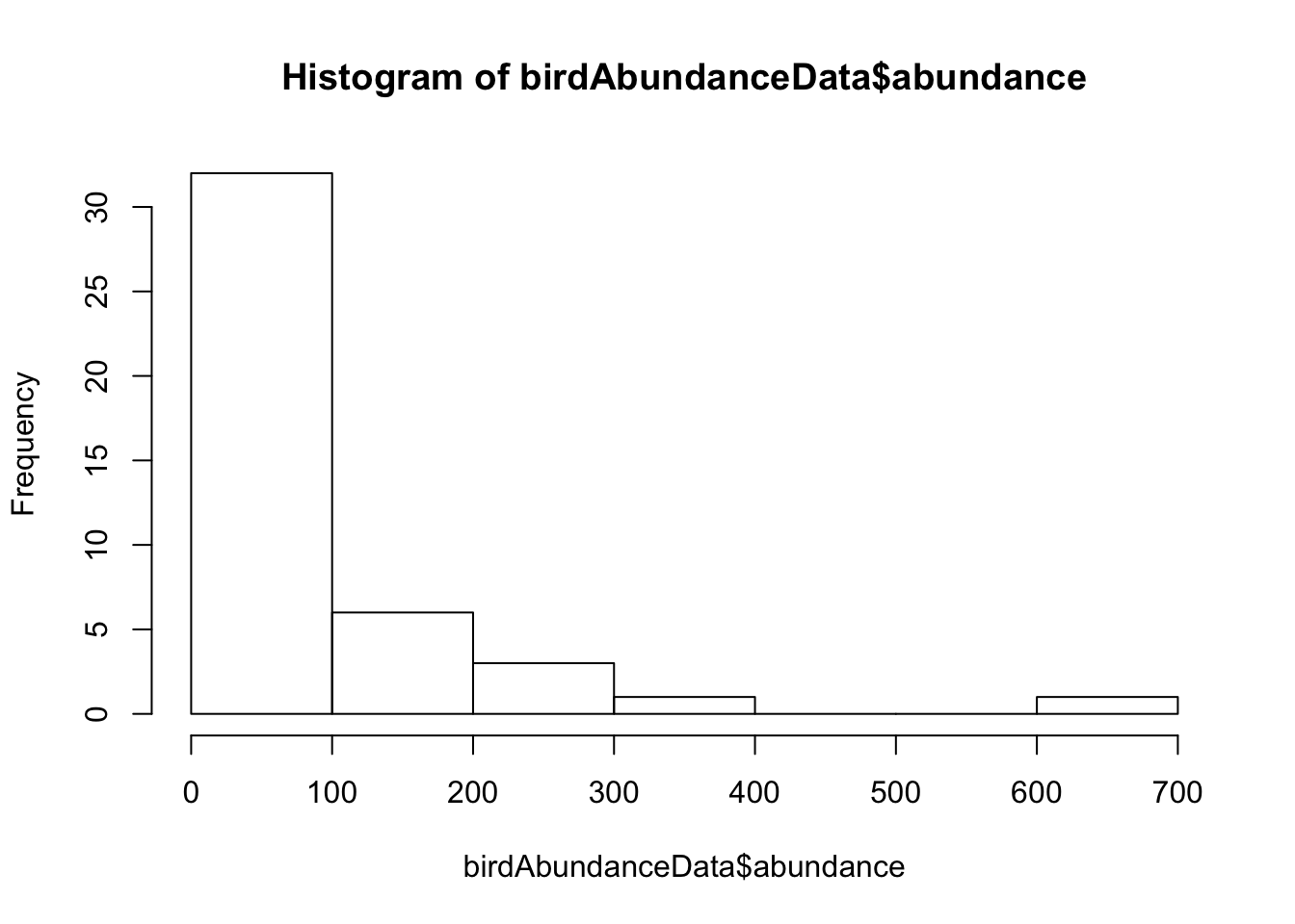
When creating histograms of non-categorical data (eg. temperature, number of amino acids in proteins), you have to specify the bins with an interval. Right = FALSE means that the histogram cells / bins are left-closed (right open) intervals: [included….not included)
How to make a scatterplot:
mydata   = data.frame(x = rnorm(100))
# in this line you're creating a data frame with a variable x, where you generate this x by randomly sampling 100 values from a normal distribution

mydata$y = 5 * mydata$x + 11.0 + rnorm(100)
# mydata$y appends another column (variable) to your dataframe
# the expression after "=" just means that this y variable is populated by values that are 5 * corresponding x + 11 + a value randomly sampled from a normal distribution
summary(mydata)
## x y
## Min. :-2.2142 Min. :-0.7026
## 1st Qu.:-0.7228 1st Qu.: 7.0930
## Median :-0.1858 Median :10.0894
## Mean :-0.0886 Mean :10.5803
## 3rd Qu.: 0.5955 3rd Qu.:14.2987
## Max. : 2.4374 Max. :22.6877head(mydata) # you can see the first couple lines of your data frame - useful for seeing what kind of variables you have ## x y
## 1 2.43743400 22.6876836
## 2 1.16356595 15.8399967
## 3 -1.30852100 3.1416905
## 4 0.09823519 13.2783280
## 5 -2.21418942 0.6249789
## 6 -1.44059181 4.7081643plot(x = mydata$x, y = mydata$y) # it's good to specify which data you want on the x axis and which to put on the y axis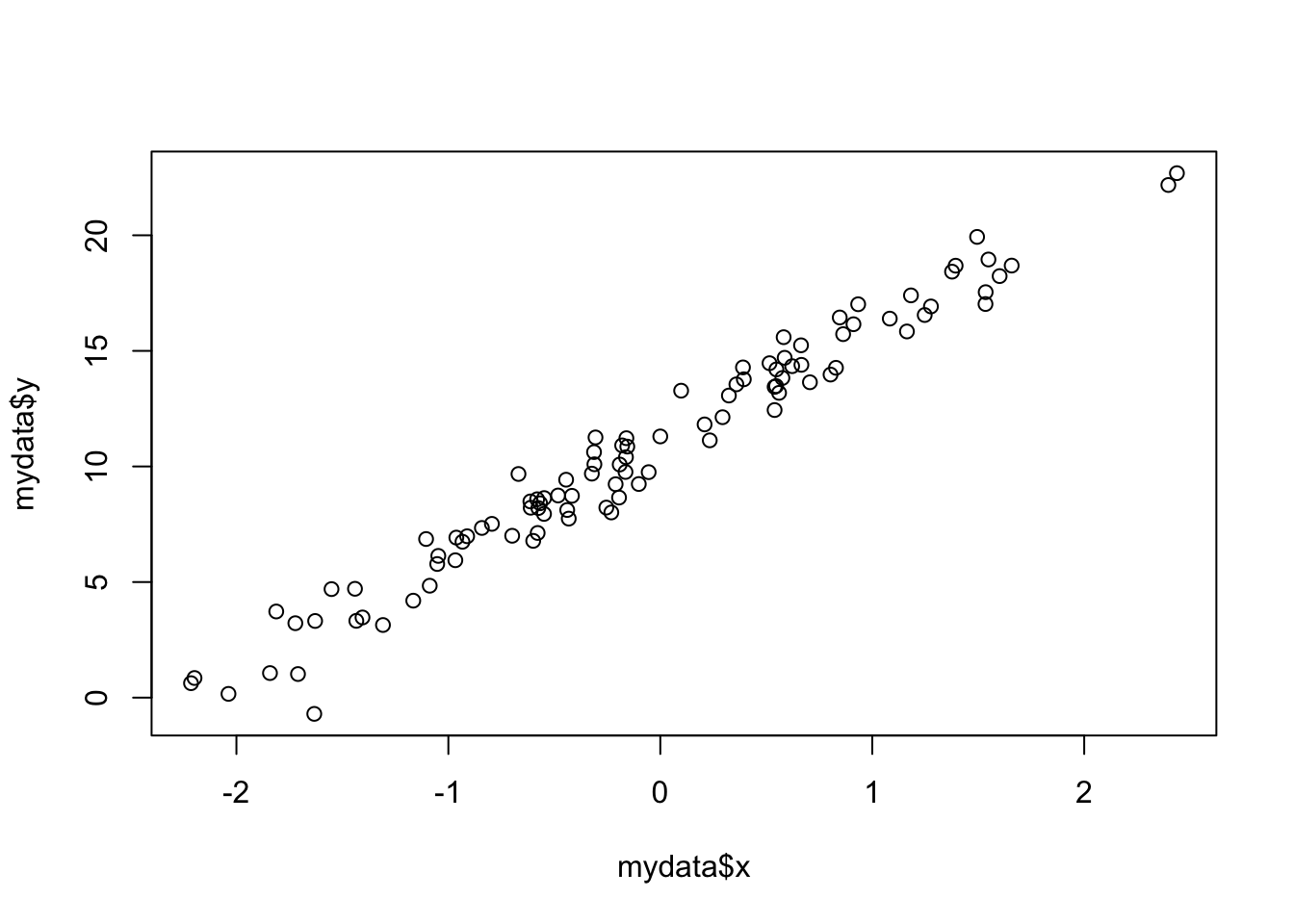
Take me back to the beginning!
The guppy dataset
Find the guppy dataset from chapter 2 and make a plot similar to figure 2.3-3
Use read.csv to read the data into a variable called Guppies:
guppies <- read.csv("chap02e3bGuppyFatherSonAttractiveness.csv")Summarize the dataset - what are the variables called and how many variables are in the dataset?
summary(guppies)## fatherOrnamentation sonAttractiveness
## Min. :0.0300 Min. :-0.3200
## 1st Qu.:0.3275 1st Qu.: 0.1800
## Median :0.4550 Median : 0.4500
## Mean :0.4908 Mean : 0.4872
## 3rd Qu.:0.6100 3rd Qu.: 0.8025
## Max. :1.1200 Max. : 1.2300The variables are called:
colnames(guppies)## [1] "fatherOrnamentation" "sonAttractiveness"There are 2 variables, fatherOrnamentation and sonAttractiveness.
Create the plot:
plot(guppies$fatherOrnamentation, guppies$sonAttractiveness) 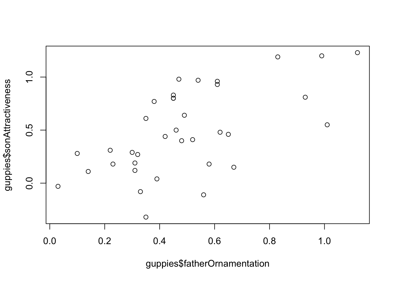
A fancier version:
plot(guppies$fatherOrnamentation, guppies$sonAttractiveness, col = "deeppink4", pch=16, xlab="Father's Ornamentation", ylab="Son's Attractiveness") 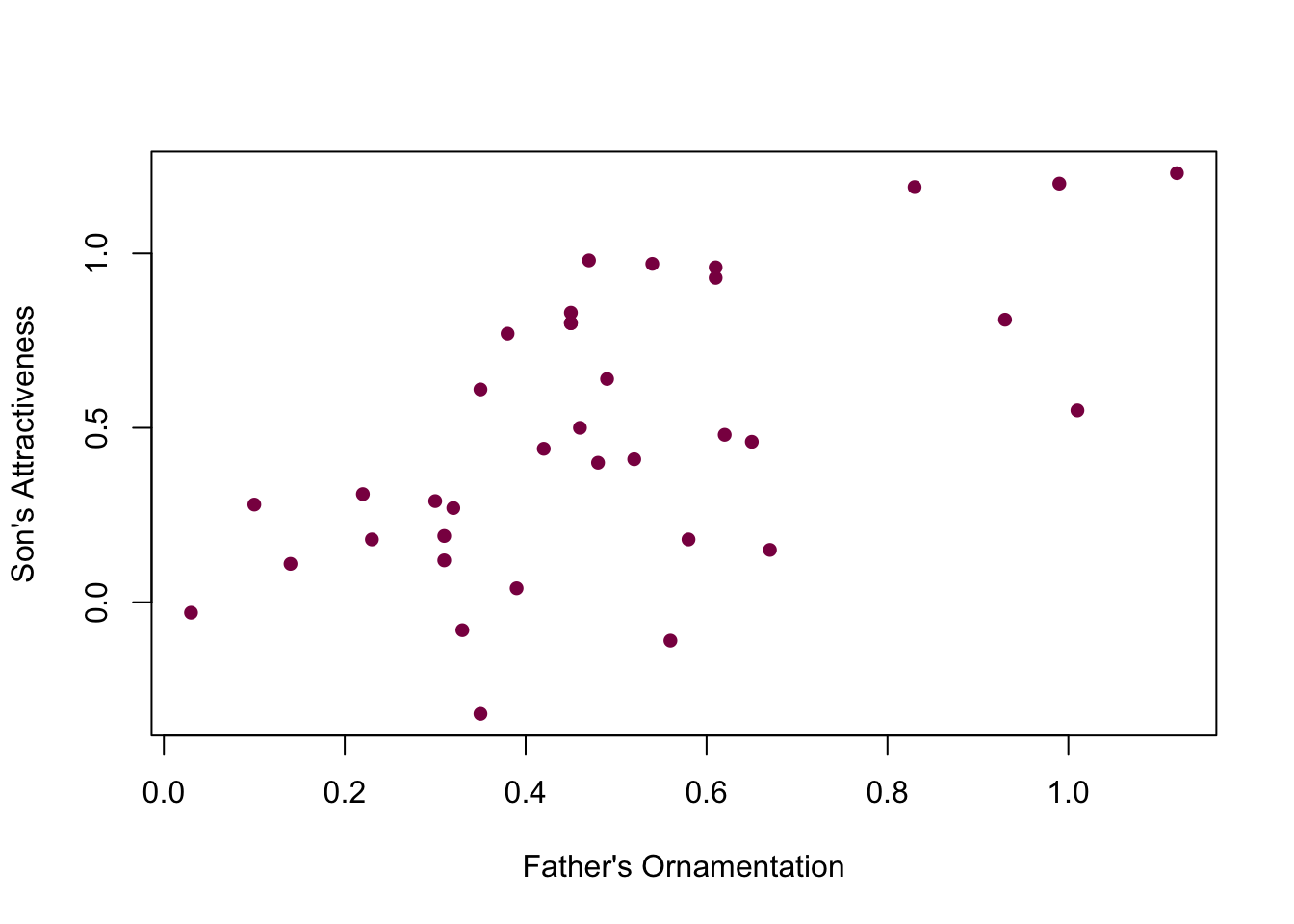
#pch = 16: determines the filled circlesTake me back to the beginning!